Ajuste Fino - Fine-Tuning

 1 - https://arxiv.org/abs/1902.03928 

The Degree of Fine-Tuning in our Universe -- and Others

Astrofísica > Cosmologia e Astrofísica Não Galáctica

[Enviado em 11 de fevereiro de 2019]

O Grau de Ajuste Fino em nosso Universo -- e Outros

Fred C. Adams

(resumido) Tanto as constantes fundamentais que descrevem as leis da física quanto os parâmetros cosmológicos que determinam as propriedades cósmicas devem estar dentro de uma faixa de valores para que o universo desenvolva estruturas astrofísicas e, por fim, suporte a vida. Este artigo analisa as restrições atuais sobre essas grandezas. O modelo padrão da física de partículas contém constantes de acoplamento e massas de partículas, e as faixas permitidas desses parâmetros são discutidas primeiro. Em seguida, consideramos os parâmetros cosmológicos, incluindo a densidade total de energia, a densidade de energia do vácuo, a razão bárion-fóton, a contribuição da matéria escura e a amplitude das flutuações de densidade primordial. Essas grandezas são restringidas pelos requisitos de que o universo viva por um longo tempo, emerja da época da BBN com uma composição química aceitável e possa produzir galáxias com sucesso. Em escalas menores, estrelas e planetas devem ser capazes de se formar e funcionar. As estrelas devem ter vidas úteis suficientemente longas e temperaturas superficiais elevadas. Os planetas devem ser massivos o suficiente para manter uma atmosfera, pequenos o suficiente para permanecerem não degenerados e conter partículas suficientes para sustentar uma biosfera complexa. Esses requisitos impõem restrições à constante gravitacional, à constante de estrutura fina e aos parâmetros compostos que especificam as taxas de reação nuclear. Consideramos casos específicos de possível ajuste fino em estrelas, incluindo a reação alfa tripla que produz carbono, bem como os efeitos do deutério instável e dos diprótons estáveis. Para todas essas questões, existem universos viáveis em uma faixa de espaço de parâmetros, que é delineada aqui. Finalmente, para universos com parâmetros significativamente diferentes, novos tipos de processos astrofísicos podem gerar energia e sustentar a habitabilidade.

Comentários: 212 páginas, 36 figuras, aceito para publicação em Physics Reports

Assuntos: Cosmologia e Astrofísica Não Galáctica (astro-ph.CO) ; Física de Altas Energias - Fenomenologia (hep-ph); Física de Altas Energias - Teoria (hep-th)

Citar como: arXiv:1902.03928 [astro-ph.CO]

  (ou arXiv:1902.03928v1 [astro-ph.CO] para esta versão)

 

https://doi.org/10.48550/arXiv.1902.03928

Concentre-se em aprender mais

DOI relacionado :

https://doi.org/10.1016/j.physrep.2019.02.001

Concentre-se em aprender mais

https://www.sciencedirect.com/science/article/abs/pii/S0370157319300511

O grau de ajuste fino em nosso universo — e outros

Os links do autor abrem o painel de sobreposiçãoFred C. Adams

Mostrar mais

Adicionar ao Mendeley

Compartilhar

Citar

https://doi.org/10.1016/j.physrep.2019.02.001

Obtenha direitos e conteúdo

Resumo

Tanto as constantes fundamentais que descrevem as leis da física quanto os parâmetros cosmológicos que determinam as propriedades do nosso universo devem estar dentro de uma faixa de valores para que o cosmos desenvolva estruturas astrofísicas e, em última análise, sustente a vida. Este artigo analisa as restrições atuais sobre essas grandezas. A discussão começa com uma avaliação dos parâmetros que podem variar. O modelo padrão da física de partículas contém constantes de acoplamento e massas de partículas, e as faixas permitidas desses parâmetros são discutidas primeiro. Em seguida, consideramos os parâmetros cosmológicos, incluindo a densidade energética total do universo.

, a contribuição da energia do vácuo

, a razão bárion-fóton

, a contribuição da matéria escura

, e a amplitude das flutuações da densidade primordial

Essas quantidades são limitadas pelos requisitos de que o universo viva por um tempo suficientemente longo, emerja da época da Nucleossíntese do Big Bang com uma composição química aceitável e possa produzir com sucesso estruturas em grande escala, como galáxias. Em escalas menores, estrelas e planetas devem ser capazes de se formar e funcionar. As estrelas devem ter vida suficientemente longa, temperaturas superficiais suficientemente altas e massas menores do que suas galáxias hospedeiras. Os planetas devem ser massivos o suficiente para manter uma atmosfera, mas pequenos o suficiente para permanecerem não degenerados, e conter partículas suficientes para sustentar uma biosfera de complexidade suficiente. Esses requisitos impõem restrições à constante gravitacional da estrutura.

, a constante de estrutura fina

, e parâmetros compostos

que especificam as taxas de reação nuclear. Em seguida, consideramos casos específicos de possível ajuste fino na nucleossíntese estelar , incluindo a reação alfa tripla que produz carbono, o caso do deutério instável e a possibilidade de diprótons estáveis. Para todas as questões descritas acima, universos viáveis existem em uma faixa de espaço de parâmetros, que é delineada aqui. Finalmente, para universos com parâmetros significativamente diferentes, novos tipos de processos astrofísicos podem gerar energia e, assim, sustentar a habitabilidade.

Introdução

As leis da física em nosso universo sustentam o desenvolvimento e as operações da biologia – e, portanto, dos observadores – que, por sua vez, requerem a existência de uma gama de estruturas astrofísicas. O cosmos sintetiza núcleos leves durante sua história inicial e, posteriormente, produz uma grande variedade de estrelas, que forjam as entradas restantes da tabela periódica. Em escalas maiores, as galáxias se condensam a partir do universo em expansão e fornecem poços profundos de potencial gravitacional que coletam e organizam os ingredientes necessários. Em escalas menores, os planetas se formam ao lado de suas estrelas hospedeiras e fornecem ambientes adequados para a gênese e a manutenção da vida. Em nosso universo, as leis da física têm a forma adequada para sustentar todos esses blocos de construção necessários para o surgimento de observadores. No entanto, um grande e crescente corpo de pesquisas tem argumentado que mudanças relativamente pequenas nas leis da física poderiam tornar o universo incapaz de suportar vida. Em outras palavras, o universo poderia ser ajustado para o desenvolvimento da complexidade. O objetivo geral desta contribuição é revisar os argumentos atuais sobre o possível ajuste fino do universo e fazer uma avaliação quantitativa de sua gravidade.

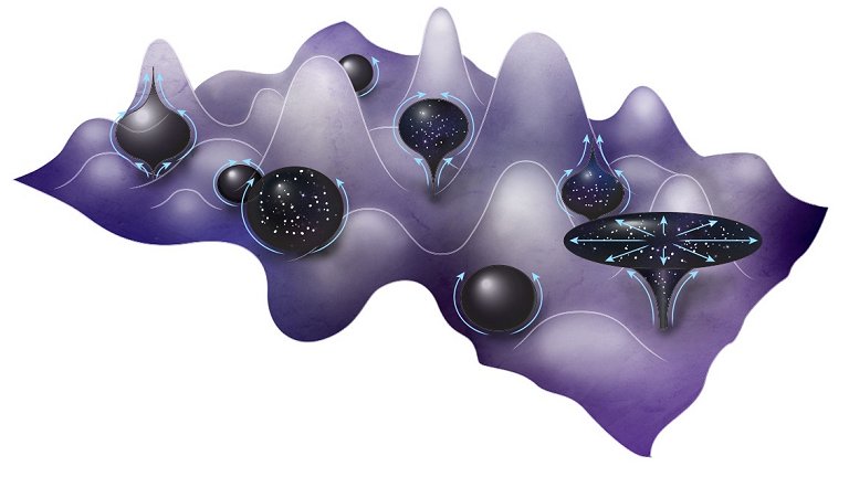
As teorias cosmológicas atuais argumentam que nosso universo pode ser apenas um componente de uma vasta coleção de universos que compõem uma região muito maior do espaço-tempo, frequentemente chamada de “multiverso” ou “megaverso” [1], [2], [3], [4], [5], [6], [7], [8], [9]. Esse conjunto é representado esquematicamente na Fig. 1. Desenvolvimentos paralelos na teoria das cordas e suas generalizações indicam que a estrutura de vácuo do universo poderia ser amostrada a partir de um enorme número de estados possíveis [10], [11], [12], [13], [14], [15]. A função de energia potencial para esse espaço de configuração é representada esquematicamente na Fig. 2, onde cada mínimo corresponde a um universo diferente de baixa energia. Se cada universo individual dentro do multiverso (representado por uma bolha específica na Fig. 1) amostrar a distribuição subjacente de possíveis estados de vácuo (escolhendo um mínimo local específico representado na Fig. 2), as leis da física poderiam variar de região para região dentro do conjunto. Nesse cenário, nosso universo representa um pequeno subdomínio de todo o espaço-tempo com uma implementação específica das versões possíveis das leis da física. Outros domínios poderiam ter partículas elementares com propriedades e/ou parâmetros cosmológicos diferentes. Surge então uma questão fundamental: quais versões das leis da física são necessárias para o desenvolvimento de estruturas astrofísicas, que por sua vez são necessárias para o desenvolvimento da vida?

Os argumentos do ajuste fino têm uma longa história [22], [23], [24], [25]. Embora muitos tratamentos anteriores tenham concluído que o universo é ajustado fino para o desenvolvimento da vida [14], [26], [27], [28], [29], [30], [31], [32], [33], [34], [35], [36], [37], [38], [39], [40], deve-se enfatizar que diferentes autores fazem essa afirmação com graus de convicção amplamente variados (ver também [2], [12], [41], [42], [43], [44], [45], [46]). Também observamos que este tópico foi abordado através das lentes da filosofia (ver [47], [48], [49], [50], [51] e referências nela contidas), embora esta discussão atual se concentre em resultados da física e da astronomia. Em qualquer caso, o conceito de ajuste fino não é definido com precisão. Aqui começamos a discussão fazendo a distinção entre dois tipos de problemas de ajuste:

O significado usual de "ajuste fino" é que pequenas mudanças no valor de um parâmetro podem levar a mudanças significativas no sistema como um todo. Por exemplo, se a força nuclear forte fosse um pouco mais fraca, o núcleo de deutério não estaria mais ligado. Se a força forte fosse um pouco mais forte, os diprótons estariam ligados. Em ambos os exemplos, mudanças relativamente pequenas (aqui, variações de vários pontos percentuais na força forte) levam a inventários nucleares diferentes. Um segundo tipo de ajuste surge quando um parâmetro de interesse tem um valor muito diferente do esperado (geralmente em bases teóricas). A constante cosmológica fornece um exemplo desse problema: o valor observado da constante cosmológica é menor do que algumas expectativas de seu valor por ordens de grandeza. Este segundo tipo de ajuste é, portanto, hierárquico. 

No primeiro exemplo, a força nuclear forte pode aparentemente variar apenas por cento sem tornar o deutério instável ou os diprótons estáveis. A estrutura nuclear representa, portanto, uma possível instância de Ajuste Fino Sensível . 

No segundo exemplo, o valor da constante cosmológica poderia ser um milhão de vezes menor ou maior (se a amplitude de flutuação também pode variar) e nada catastrófico aconteceria, mas os valores ainda seriam muito menores do que a escala de Planck (por ordens de magnitude ou mais). A constante cosmológica é, portanto, um exemplo de Ajuste Fino Hierárquico .

Além disso, quando surge uma hierarquia inesperada devido a alguma quantidade ser muito menor do que sua escala natural, uma maneira de obter tal ordenação é que dois números grandes quase, mas não completamente, se cancelem. Esse quase cancelamento de grandes quantidades pode ser extremamente sensível aos seus valores exatos e, portanto, pode exigir algum tipo de ajuste. Esse estado de coisas surge, por exemplo, no problema da constante cosmológica [52], [53] (ver Seção 4). Esse conceito geral é conhecido como Naturalidade . Embora existam muitas definições na literatura, a ideia básica é que uma quantidade na física de partículas é considerada não natural se as correções quânticas forem maiores do que o valor observado (para discussões recentes sobre esse assunto, ver [54], [55] e referências nele contidas; para um ponto de vista mais crítico, ver [56]). Em tal situação, as correções quânticas devem (principalmente) se cancelar para permitir que o pequeno valor observado surja. Esse cancelamento não é automático, de modo que requer alguma medida de ajuste fino. Uma maneira de codificar esse conceito, devido a 't Hooft, é declarar um Princípio de Naturalidade: Uma quantidade física deve ser pequena se e somente se a teoria subjacente se torna mais simétrica no limite onde essa quantidade se aproxima de zero [57].

Os constituintes físicos do nosso universo apresentam uma hierarquia de escalas que lhe permite funcionar [30], [45], [58]. Antes de considerar os detalhes do ajuste fino, é útil avaliar o escopo do nosso universo em particular. A Figura 3 ilustra a gama de escalas de comprimento e massa que permitem o funcionamento do nosso universo. As massas e os comprimentos são dados em unidades de massa do próton e de tamanho do próton, respectivamente. O símbolo triangular na origem marca assim a localização do próton. Na outra extremidade do diagrama, a massa e o tamanho do universo observável são marcados pelo triângulo em Objetos que são menores que seus horizontes de eventos () caem abaixo da linha vermelha e se encontram no regime do buraco negro. Objetos que são menores que seus comprimentos de onda Compton () caem abaixo da linha azul e se encontram no regime quântico. Essas duas regiões se encontram na localização de um buraco negro de massa de Planck, marcado pelo triângulo inferior em

. Contornos de densidade constante são mostrados pelas linhas tracejadas na figura. Vários corpos macroscópicos situam-se perto da linha de densidade atômica (curva tracejada do meio), que se estende do átomo de hidrogênio à esquerda até o limite do buraco negro à direita. No meio, o segmento de linha verde mostra o regime de formas de vida conhecidas, variando de bactérias a baleias. Planetas são representados pelos símbolos quadrados e estrelas são representadas pelos círculos. O intervalo de buracos negros conhecidos é mostrado pelo segmento de linha preta grossa. Observe que este segmento é muito menor do que o intervalo total possível de buracos negros, que poderia abranger toda a linha vermelha. Finalmente, a região amostrada por estruturas galácticas é mostrada como a região sombreada na parte superior direita do diagrama.

A Fig. 3 ilustra tanto os desafios quanto as limitações impostas pelas escalas do universo. A amplitude total da massa abrange aproximadamente 80 décadas. A amplitude na escala radial, embora ampla, é mais restrita. A curva tracejada inferior mostra o contorno da densidade nuclear. Em grandes escalas de massa, onde a gravidade pode comprimir o material até atingir densidades mais altas, os objetos se tornam buracos negros. Para massas menores, as forças nucleares dominam, de modo que nosso universo geralmente não produz entidades com tamanhos abaixo da linha de densidade nuclear. A curva tracejada superior corresponde à densidade do universo como um todo. Objetos acima dessa curva teriam densidades menores que a do espaço de fundo e estariam sujeitos à destruição por maré. Como resultado, nosso universo geralmente não produz entidades que se situem acima dessa linha. A amplitude de tamanhos possíveis para uma dada massa, portanto, abrange "apenas" cerca de 15 décadas (com uma amplitude menor em massas elevadas devido ao limite do buraco negro). O universo, com sua estrutura multifacetada, suporta um espaço de parâmetros com extensão de cerca de 80 × 15 décadas. Essa ampla gama de escalas de comprimento e massa é possibilitada pela ampla hierarquia entre a força da gravidade e a força eletromagnética. Como enfatizado anteriormente [30], [45], se a gravidade fosse mais forte, essa gama de escalas seria correspondentemente menor: a linha vermelha se moveria para cima na Figura 3 e o espaço disponível para estruturas astrofísicas diminuiria consequentemente.

Outra característica do universo ilustrada pela Figura 3 é que as regiões ocupadas por tipos específicos de objetos terrestres e astrofísicos são relativamente pequenas. O diagrama mostra as localizações no espaço de parâmetros povoadas por formas de vida, planetas, estrelas, buracos negros e galáxias. Além disso, as regiões povoadas por átomos estão densamente agrupadas perto do ponto mostrado para o átomo de hidrogênio. Da mesma forma, os núcleos estão agrupados perto da localização do próton. Todas essas regiões são pequenas em comparação com o espaço de parâmetros total disponível e estão amplamente separadas umas das outras.

A questão central em análise é se os parâmetros da física em nosso universo estão ajustados com precisão para o desenvolvimento da vida. Essa questão, que pode ser formulada de forma simples, é repleta de complicações. Esta seção descreve os componentes básicos do problema do ajuste fino.

O primeiro passo é especificar quais parâmetros da física e da astrofísica podem variar de universo para universo. É bem conhecido que o Modelo Padrão da Física de Partículas possui pelo menos 26 parâmetros, mas a teoria deve ser estendida para levar em conta aspectos físicos adicionais, incluindo gravidade, oscilações de neutrinos, matéria escura e energia escura (Seção 2). A especificação de tais extensões requer parâmetros adicionais. Por outro lado, nem todos os parâmetros são necessariamente vitais para o funcionamento do universo de baixa energia (que não depende das massas exatas dos quarks pesados). Uma esperança – ainda não concretizada – é que uma teoria mais fundamental teria menos parâmetros e que o grande número de parâmetros do Modelo Padrão poderia ser derivado ou calculado a partir do conjunto menor. Como resultado, o número de parâmetros poderia ser maior ou menor do que os 26 conhecidos. Além dos parâmetros da física de partículas, o Modelo Cosmológico Padrão possui seu próprio conjunto de grandezas necessárias para especificar as propriedades do universo (Seção 3). 

Esses parâmetros incluem a razão bárion-fóton., a proporção análoga para a matéria escura, a amplitude

das flutuações da densidade primordial, a densidade de energia do espaço de fundo, e assim por diante.

 Em princípio, algumas ou todas essas grandezas poderiam ser calculadas a partir de uma teoria fundamental, mas esse programa não pode ser executado no momento. Mesmo que os parâmetros cosmológicos sejam calculáveis, seus valores poderiam depender da história de expansão do universo específico em questão, de modo que esses valores dependem das condições iniciais (presumivelmente estabelecidas na época de Planck).

Uma vez identificados os parâmetros ajustáveis da física e da cosmologia, uma descrição completa do problema deve considerar suas distribuições de probabilidade. 

No caso de um único parâmetro, precisamos conhecer a distribuição de probabilidade subjacente de um universo para obter um determinado valor desse parâmetro. Por exemplo, se a distribuição de probabilidade subjacente for uma função delta, que seria centrada no valor medido em nosso universo, então todos os universos devem ser os mesmos nesse aspecto. No caso mais geral de interesse para argumentos de ajuste fino, as distribuições de probabilidade são consideradas suficientemente amplas para que grandes desvios do nosso universo sejam possíveis. Em particular, a faixa de valores possíveis dos parâmetros (os mínimos e máximos das distribuições) deve ser especificada. Uma avaliação completa do ajuste fino requer o conhecimento dessas distribuições de probabilidade fundamentais, uma para cada parâmetro de interesse (embora não sejam necessariamente independentes). Infelizmente, essas distribuições de probabilidade não estão disponíveis no momento.

As distribuições de probabilidade descritas acima são a priori, ou seja, distribuições teoricamente previstas que se aplicam a um ponto aleatório no espaço-tempo no final da época inflacionária (ou, mais genericamente, qualquer época do universo ultra-inicial que estabeleça suas condições iniciais). Conforme enfatizado pela Ref. [59], também é preciso considerar os efeitos de seleção para testar as previsões teóricas por meio de experimentos. Por exemplo, se um parâmetro afeta a formação de planetas, a distribuição de probabilidade para esse parâmetro será diferente quando avaliada em um ponto aleatório no espaço-tempo ou em um planeta aleatório.

O próximo passo crucial é determinar qual a gama de parâmetros que permite o desenvolvimento de observadores. A questão do que constitui um observador representa mais uma complicação. Para fins de precisão, esta revisão considera um universo bem-sucedido (equivalentemente viável ou habitável) se puder suportar toda a gama de estruturas astrofísicas necessárias para o surgimento da vida ou de algum tipo de complexidade. Assumimos então implicitamente que observadores surgirão se as estruturas necessárias estiverem presentes, e não nos preocuparemos se os observadores resultantes são ratos, golfinhos ou androides. A lista de estruturas necessárias inclui núcleos complexos, planetas, estrelas, galáxias e o próprio universo. Além de sua existência, essas estruturas devem ter as propriedades corretas para suportar observadores. Núcleos estáveis devem povoar uma fração adequada da tabela periódica. As estrelas devem ser suficientemente quentes e viver por um longo período. As galáxias devem ter poços de potencial gravitacional profundos o suficiente para reter elementos pesados produzidos pelas estrelas e não excessivamente densos para que os planetas possam permanecer em órbita. O próprio universo deve permitir que as galáxias se formem e vivam por tempo suficiente para que a complexidade surja. E assim por diante. A maior parte desta revisão descreve as restrições aos parâmetros da física e da astrofísica impostas por esses requisitos.

Para resumir esta discussão: para fazer uma avaliação completa do grau de ajuste fino do universo, é preciso abordar os seguintes componentes do problema:

[

] Especificação dos parâmetros relevantes da física e astrofísica que podem variar de universo para universo.

[

] Determinação dos intervalos permitidos de parâmetros que permitem o desenvolvimento da complexidade e, portanto, dos observadores.

[

] Identificação das distribuições de probabilidade subjacentes das quais os parâmetros fundamentais são extraídos, incluindo todo o intervalo possível que os parâmetros podem assumir.

[

] Consideração de efeitos de seleção que permitem a interpretação de propriedades observadas no contexto das distribuições de probabilidade a priori .

[

] Síntese dos ingredientes anteriores para determinar a probabilidade geral dos universos se tornarem habitáveis.

Este tratamento concentra-se principalmente nas duas primeiras considerações. Tanto para o Modelo Padrão da Física de Partículas quanto para o atual Modelo de Consenso da Cosmologia, revisamos o conjunto completo de parâmetros e identificamos aqueles que têm maior influência na determinação da habitabilidade potencial do universo. A maior parte do manuscrito, então, revisa as restrições impostas às faixas permitidas dos parâmetros relevantes, exigindo que o universo possa produzir e manter estruturas complexas. Infelizmente, as distribuições de probabilidade subjacentes não são conhecidas nem para os parâmetros fundamentais da física nem para os parâmetros cosmológicos. Como resultado, essas distribuições e como elas influenciam os efeitos de seleção são considerados apenas brevemente. Da mesma forma, os efeitos de seleção dependem das distribuições de probabilidade para os parâmetros fundamentais e não podem ser adequadamente abordados neste momento.

A consideração de possíveis universos alternativos, aqui com diferentes encarnações das leis da física, é, por definição, um empreendimento contrafactual. Esta revisão considera as faixas de parâmetros físicos que permitem que tal universo seja viável. Como universos alternativos não são observáveis, esse esforço necessariamente se situa próximo dos limites da ciência [1], [5]. No entanto, esta discussão é útil em várias frentes: primeiro, pode-se levar a sério a existência do multiverso, de modo que outros universos sejam considerados como realmente existentes, e a questão de sua possível habitabilidade seja relevante [9]. Além disso, se a teoria do multiverso se tornar suficientemente desenvolvida, então, em princípio, poder-se-ia prever a probabilidade de um universo ter uma realização particular das leis da física e, portanto, estimar a probabilidade de um universo se tornar habitável. Em segundo lugar, argumentos antrópicos [28], [30] estão sendo usados atualmente como explicação para o motivo pelo qual o universo tem sua versão observada das leis da física. Para compreender ambas as questões, o primeiro passo é determinar as faixas de parâmetros que permitem que um universo desenvolva estrutura e complexidade. Por fim, e talvez o mais importante, estudar o grau de ajuste necessário para o universo operar nos proporciona uma maior compreensão de como ele funciona.

Nesta revisão, o termo multiverso refere-se ao conjunto de outros universos possíveis representados esquematicamente na Figura 1 — outras regiões do espaço-tempo que são distantes e amplamente desconectadas do nosso próprio universo. Para completar, notamos que a Interpretação de Muitos Mundos da mecânica quântica [60], [61] descreve a realidade física como bifurcando-se em múltiplas cópias de si mesma, e essa coleção de possibilidades às vezes também é chamada de multiverso [3]. Aqui, consideramos o multiverso apenas no primeiro sentido, cosmológico. A filosofia da mecânica quântica e, portanto, o segundo tipo de multiverso, está além do escopo deste tratamento.

Esta revisão está organizada da seguinte forma: consideramos inicialmente o Modelo Padrão da Física de Partículas na Seção 2. Após discutir toda a gama de parâmetros, focamos no subconjunto de grandezas que têm maior influência na determinação das propriedades de estruturas complexas e, em seguida, discutimos as restrições sobre esses parâmetros, resultantes principalmente de considerações da física de partículas. Restrições adicionais resultantes de requisitos astrofísicos são discutidas nas seções subsequentes. O Modelo Padrão da Cosmologia é apresentado na Seção 3. Toda a gama de parâmetros cosmológicos é revisada, juntamente com uma avaliação das grandezas mais importantes para a produção de estrutura e algumas restrições básicas sobre o inventário cósmico. O caso da constante cosmológica (energia escura) é de particular interesse e é considerado separadamente na Seção 4. A época da Nucleossíntese do Big Bang (BBN) também é considerada separadamente na Seção 5, que avalia como as abundâncias dos elementos leves mudam com a variação dos valores dos parâmetros cosmológicos de entrada. A formação de galáxias e a estrutura galáctica são consideradas na Seção 6, que fornece restrições sobre parâmetros fundamentais e cosmológicos devido às propriedades galácticas necessárias. A Seção 7 considera as restrições devido à necessidade de estrelas em funcionamento, que são necessárias para ter configurações de queima nuclear estáveis, vidas úteis suficientemente longas e fotosferas quentes. Esta seção também revisita as questões clássicas da ressonância alfa tripla para a produção de carbono, os efeitos do deutério instável e os efeitos dos diprótons estáveis. As propriedades necessárias dos planetas são consideradas na Seção 8, onde as restrições de parâmetros são semelhantes – mas menos limitantes – às de considerações estelares. Cenários mais exóticos são introduzidos na Seção 9, incluindo fontes alternativas de geração de energia, como a aniquilação da matéria escura e a radiação de buracos negros. O artigo conclui na Seção 10 com um resumo das restrições de ajuste fino e uma discussão de suas implicações. Uma série de Apêndices fornece uma discussão mais aprofundada e apresenta algumas questões auxiliares, incluindo um resumo das escalas de massa astrofísica em termos das constantes fundamentais Apêndice A, o número de dimensões espaço-temporais Apêndice B, bioquímica molecular Apêndice C, limites globais nas constantes de estrutura Apêndice D, uma breve discussão das distribuições de probabilidade subjacentes para os parâmetros ajustáveis Apêndice E e o intervalo de núcleos possíveis Apêndice F.

Uma nota sobre a notação: A literatura da física de partículas geralmente usa unidades naturais onde

,

, e

A maior parte da nossa discussão sobre tópicos de física de partículas segue essa convenção. Por outro lado, a maior parte da literatura astrofísica usa unidades CGS, portanto, a discussão sobre estrelas e planetas inclui os fatores relevantes de

e

.

Acesso através da sua organização

Verifique o acesso ao texto completo fazendo login na sua organização.

Trechos de seção

Parâmetros da física de partículas

Uma avaliação completa dos parâmetros da física de partículas – juntamente com uma análise do seu possível grau de ajuste fino – é dificultada pelo atual estado de desenvolvimento da área. Por um lado, o Modelo Padrão da Física de Partículas fornece uma descrição notavelmente bem-sucedida da maioria dos resultados experimentais até o momento. Além de seus inúmeros sucessos, a teoria é elegante e bem fundamentada. Por outro lado, esta teoria é incompleta. Já sabemos que extensões ao modelo mínimo

Parâmetros cosmológicos e o inventário cósmico

Esta seção descreve os parâmetros cosmológicos necessários para descrever um universo como membro do multiverso. Começamos com uma revisão dos parâmetros cosmológicos necessários para especificar o estado atual do nosso próprio universo. No entanto, alguns desses parâmetros têm relativamente pouco efeito na formação da estrutura e não são necessários para que um universo arbitrário seja habitável. Assim, definimos o subconjunto de parâmetros relevantes para considerações de ajuste fino em todo o universo.

A constante cosmológica e/ou energia escura

Embora nosso universo possa ser especificado por relativamente poucos parâmetros cosmológicos (ver Seção 3), um dos ingredientes necessários é uma densidade energética substancial do vácuo — frequentemente chamada de energia escura. Essa quantidade atua como uma constante cosmológica e é atualmente o componente dominante do inventário cósmico (ver Tabela 1). A energia escura está impulsionando a aceleração observada atualmente no universo e terá enormes consequências no futuro [204], [205], [206]. Além disso, a

Nucleossíntese do Big Bang

Para que um universo se torne habitável, ele deve produzir núcleos complexos com sucesso. Em nosso universo, a nucleossíntese ocorre em múltiplos cenários, incluindo o universo primordial, núcleos estelares, explosões de supernovas e espalação no meio interestelar. Nos primeiros minutos de sua história, nosso universo processa cerca de um quarto de seu material bariônico em hélio-4 durante uma época conhecida como Nucleossíntese do Big Bang (BBN). Embora as estrelas também produzam hélio, esse processamento inicial

Formação de galáxias e estrutura em larga escala

As galáxias são componentes vitais de um universo habitável. Elas coletam e organizam o gás interestelar necessário para a formação de estrelas, que fornecem a energia e os núcleos pesados necessários para o desenvolvimento biológico. De igual importância, as galáxias devem ter massa suficiente para reter os elementos pesados produzidos pela nucleossíntese estelar. Para cumprir essas funções, as galáxias devem primeiro ser capazes de se formar.

A formação de galáxias envolve uma série de processos físicos (ver [248] para uma revisão recente e 

Estrelas e evolução estelar

As estrelas desempenham dois papéis importantes em relação à habitabilidade do nosso universo, e presumivelmente outros. Primeiro, elas fornecem a maior parte da energia [150] disponível para sustentar biosferas em quaisquer planetas convenientemente situados. Segundo, elas forjam a maioria dos núcleos pesados necessários para o desenvolvimento de estruturas complexas [296], [297], que vão desde os próprios planetas até entidades biológicas.

Planetas

Os planetas representam os menores objetos astrofísicos necessários para o desenvolvimento da vida (como a conhecemos). Para que um determinado universo se torne habitável, as leis da física devem permitir a produção de planetas com uma série de propriedades básicas, conforme descrito nesta seção. Esses corpos devem ter massa suficientemente pequena para que não se degenerem. Este requisito também é necessário (mas não suficiente) para que o planeta tenha uma superfície sólida [374]. Por outro lado, a

Cenários astrofísicos exóticos

Nossa bolha local de espaço paramétrico é adequada para habitabilidade, e a discussão até agora se concentrou em delinear os limites dessa região. Dada a ampla gama de parâmetros da física de partículas e cosmológicos que poderiam ser realizados em todo o multiverso, torna-se possível que outros universos utilizem caminhos e fontes de energia não convencionais. Como resultado, bolhas adicionais de habitabilidade poderiam existir com propriedades cósmicas marcadamente diferentes das nossas. Esta seção explora

Conclusão

Uma intrincada rede de restrições deve ser satisfeita para que um dado universo seja viável. Esta seção fornece um guia através do labirinto, organizando os resultados desta revisão de diversas maneiras: a Seção 10.1 apresenta um resumo direto dos resultados mais importantes. A Seção 10.2 identifica as tendências gerais que emergem deste conjunto de restrições. A relação com os argumentos antrópicos é abordada na Seção 10.3, e as variações de parâmetros que potencialmente permitem...

2 - https://www.inovacaotecnologica.com.br/noticias/noticia.php?artigo=ajuste-fino-universo-vida-ilusao&id=010130220209#google_vignette 

Ajuste fino do Universo para a vida pode ser uma ilusão

Com informações da Fundação John Templeton - 09/02/2022

Ajuste fino do Universo para a vida pode ser uma ilusão

Com informações da Fundação John Templeton - 09/02/2022

Um multiverso fornece uma explicação para o problema do ajuste fino, do porquê nosso cosmos parece ter os parâmetros perfeitamente ajustados para abrigar vida inteligente.

[Imagem: Maayan Harel/FQXi]

Multiverso

Nas últimas décadas, algumas das mentes mais perspicazes da física sentiu-se atraída pelo que se convencionou chamar de "problema do ajuste fino" - ou sintonia fina.

Ao sondar as leis físicas do Universo e determinar com precisão os valores das constantes físicas - como as massas das partículas elementares e as magnitudes das forças - os físicos descobriram que variações surpreendentemente pequenas nesses valores teriam criado um Universo sem vida.

Isso levou a um enigma: Por que as condições físicas do Universo são aparentemente tão bem adaptadas à existência humana?

Alguns físicos explicaram essas condições como acidentais invocando a teoria do multiverso, que propõe que há um número infinito de universos paralelos, cada um com diferentes parâmetros físicos. Dentro dessa estrutura em multiverso, não seria tão surpreendente que os humanos tenham evoluído em uma das realidades paralelas em que as condições são habitáveis para nós.

Mas muitos outros físicos permanecem céticos, tanto quanto aos multiversos quando à ideia de que nosso Universo estaria bem ajustado para a vida.

Ajuste fino desnecessário

Com o apoio do Instituto de Questões Fundamentais (FQXi) e da Fundação John Templeton, a física Miriam Frankel elaborou um extenso relatório no qual ela explora a complexa história da pesquisa sobre o ajuste fino, incluindo possíveis explicações para ela - como aquelas derivadas da teoria das cordas e do multiverso - e avaliando propostas para testar experimentalmente essas explicações direta e indiretamente.

Ocorre que o criterioso levantamento, abarcando as pesquisas mais recentes, encontrou poucas razões para que sequer seja necessário aventar o ajuste fino.

"Acontece que a sintonia necessária para que alguns desses parâmetros físicos deem origem à vida é menos precisa do que a sintonia necessária para captar uma estação em seu rádio, segundo novos cálculos," disse Frankel. "Se for verdade, o aparente ajuste fino pode ser uma ilusão."

Parece que os mecanismos fundamentais do Universo são muito mais tolerantes do que os cientistas pensavam.

[Imagem: Miriam Frankel/FQXi]

Flexibilidade do Universo

Em seu relatório, Frankel observa que a vida pode assumir uma forma muito diferente da que temos ingenuamente imaginado e que, se vários parâmetros físicos forem considerados como variando simultaneamente, essas variações podem aliviar quaisquer problemas aparentes de ajuste fino.

Isso sugere que o Universo pode não ser assim tão finamente ajustado; ele pode ser capaz de produzir vida sob uma gama muito mais ampla de circunstâncias do que se pensava inicialmente.

Por exemplo, muitas vezes foi dito que, mesmo mudanças sutis no equilíbrio das forças que governam o núcleo atômico, ou os valores das constantes fundamentais da natureza, isso poderia afetar a formação de carbono nas estrelas - necessário para o desenvolvimento da vida orgânica - ou afetaria o tempo de vida das estrelas, impedindo-as de fornecer energia suficiente para a existência de planetas habitáveis.

Mas as equações da estrutura estelar podem ter mais soluções do que a maioria das pessoas imagina.

"As estrelas podem continuar a funcionar com variações substanciais nas constantes fundamentais," disse o professor Fred Adams, astrofísico da Universidade de Michigan, cujo trabalho é analisado no relatório. "Além disso, se um processo astrofísico em particular se tornar inoperável, então (frequentemente) outro processo pode tomar seu lugar para ajudar a fornecer energia para o Universo".

"Quando os parâmetros necessários para a vida parecem aparecer em regiões suspeitamente estreitas, procuramos explicações para isso como coincidência ou conspiração cósmica. Descobrir que essas regiões podem ser mais amplas, ou que existem outras regiões que permitem a vida, enfraquece a necessidade de tais explicações. Pode ser que, no final, não haja nenhuma conspiração," disse David Sloan, físico da Universidade de Lancaster, cuja pesquisa também é apresentada no relatório.

Bibliografia:

Artigo: Fine Tuning

Autores: Miriam Frankel

Revista: FQXi Reports

Link: https://www.templeton.org/wp-content/uploads/2022/01/Fine-tuning-research-1.pdf

3 - https://www.islamreligion.com/pt/articles/10518/viewall/ajuste-fino-do-universo-parte-1-de-8 

Ajuste fino do universo (parte 1 de 8): Leis da física

https://www.islamreligion.com/pt/articles/10522/ajuste-fino-do-universo-parte-2-de-8 

Ajuste fino do universo (parte 2 de 8): Constantes & condições iniciais

https://www.islamreligion.com/pt/articles/10524/ajuste-fino-do-universo-parte-3-de-8 

Ajuste fino do universo (parte 3 de 8): Quatro exemplos de ajuste fino

https://www.islamreligion.co

m/pt/articles/10523/ajuste-fino-do-universo-parte-4-de-8 

Ajuste fino do universo (parte 4 de 8): Exemplos extremos de ajuste fino

https://www.islamreligion.com/pt/articles/10528/ajuste-fino-do-universo-parte-5-de-8 

Ajuste fino do universo (parte 5 de 8): Objeções ao ajuste fino

https://www.islamreligion.com/pt/articles/10529/ajuste-fino-do-universo-parte-6-de-8 

Ajuste fino do universo (parte 6 de 8): Como podemos explicar o ajuste fino?

https://www.islamreligion.com/pt/articles/10539/ajuste-fino-do-universo-parte-7-de-8 

Ajuste fino do universo (parte 7 de 8): Universos múltiplos

Ajuste fino do universo (parte 1 de 8): Leis da física

Classificação:

Tamanho da fonte:

Descrição: O ajuste fino é um argumento da física e cosmologia para a criação divina do universo.  Será mostrado que descobertas da física e cosmologia nos últimos cinquenta anos dão grande apoio à existência de Deus e à criação divina do universo.  Esse artigo descreverá as leis elegantes e finamente ajustadas da natureza.

Categoria:

Artigos Evidência de que o Islã é a Verdade Provas Lógicas

Categoria:

Artigos Evidência de que o Islã é a Verdade A Existência de Deus

• Por Imam Mufti (© 2016 IslamReligion.com)
• Publicado em 19 Dec 2016
• Última modificação em 30 Oct 2022
• Impresso: 54
• 'Visualizado: 21,090
• Classificação: nenhum ainda
• Classificado por: 0
• Enviado por email: 0
• Comentado em: 0

FacebookTwitterWhatsAppEmail

O que é ajuste fino?

Ao longo do século passado os cientistas descobriram que se certas propriedades do universo fossem mudadas muito ligeiramente, não estaríamos aqui.  Elas têm que estar dentro de uma faixa muito estreita para que o nosso universo torne a vida possível e seja habitável. 

O universo tem um ajuste fino para a existência de vida inteligente com uma complexidade e delicadeza que literalmente desafiam a compreensão humana.  A sensibilidade da "habitabilidade" do universo a mudanças pequenas é chamada de "ajuste fino".

Isso foi reconhecido há aproximadamente 60 anos por Fred Hoyle, que não era uma pessoa religiosa na época em que fez a descoberta.  Cientistas como Paul Davies, Martin Rees, Max Tegmark, Bernard Carr, Frank Tipler, John Barrow e Stephen Hawking, para mencionar alguns, acreditam no ajuste fino.  Esses são nomes proeminentes em cosmologia e são ouvidos na mídia toda vez que há alguma manchete.

Tipos de ajuste fino

1.  Ajuste fino das leis da natureza.

2.  Ajuste fino das constantes da física.

3.  Ajuste fino das condições iniciais do universo.

Exploraremos cada categoria abaixo:

1.  Ajuste fino das leis da natureza

Existem duas maneiras de analisar esse aspecto do ajuste fino:

1.    As leis certas que são necessárias, de maneira precisa, para que vida altamente complexa possa existir.  Se uma dessas estiver faltando, essa vida não seria possível.  Dizer que as leis são finamente ajustadas significa que o universo deve ter o conjunto certo de leis, para que vida altamente complexa possa existir.  Talvez esse tipo de ajuste fino seja o mais fácil de compreender dentre os três.

Exemplo 1: A lei da gravidade afirma que todas as massas se atraem.  Como seria o universo se a gravidade não existisse? Não haveria estrelas ou planetas.  A matéria seria distribuída igualmente em todo o universo sem lugar para vida se formar ou fontes de energia como o sol, que fornece alimento para plantas por meio da fotossíntese que, por sua vez, se tornam alimento para animais.

Exemplo 2: Um tipo de força pode desempenhar papeis múltiplos nesse sistema muito bem projetado.  Por exemplo, a força eletromagnética se refere a combinação de forças elétricas e magnéticas.  James Clerk Maxwell unificou as duas forças nos anos 1800. 

Se não houvesse força eletromagnética não haveria átomos, porque não haveria força para segurar os elétrons com carga negativa com os prótons com carga positiva, que permite as ligações químicas.  Não haveria elementos constitutivos da vida, já que não haveria ligação química e, portanto, não haveria vida. 

A força eletromagnética desempenha outro papel na luz, que é um tipo de radiação eletromagnética.  Permite que a energia se transfira do sol para o nosso planeta.  Sem essa energia, não existiríamos. 

2.    Harmonia entre natureza e matemática: Somente no século 20 passamos a entender que o que observamos na natureza pode ser descrito por algumas leis físicas, cada uma descrita por equações matemáticas simples.  É incrível fato de essas formas matemáticas serem tão simples e poucas em número a ponto de poderem ser todas escritas em uma folha de papel.

Tabela1.  As leis fundamentais da natureza

·Mecânica (Equações de Hamilton)

·Eletrodinâmica (Equações de Maxwell)

·Mecânica estatística (Equações de Boltzmann)

·Mecânica quântica (Equações de Schrödinger)

·Relatividade geral (Equação de Einstein)

Para a vida existir, precisamos de um universo ordenado e inteligível.  Além disso, é necessário ordem em muitos níveis diferentes. 

Por exemplo, para ter planetas que circulam suas estrelas, precisamos da mecânica newtoniana. 

Para haver múltiplos elementos estáveis da tabela periódica para prover uma variedade suficiente de "elementos constitutivos" atômicos para vida, precisamos da estrutura atômica dada pelas leis da mecânica quântica. 

Precisamos da ordenação nas reações químicas que é a consequência da equação de Boltzmann para a segunda lei da termodinâmica. 

E para uma fonte de energia com o sol transferir sua energia que dá vida para um habitat como a Terra, são necessárias as leis de radiação eletromagnética que Maxwell descreveu.[1]

O físico e ganhador do prêmio Nobel Eugene Wigner em seu trabalho amplamente citado The Unreasonable Effectiveness of Mathematics in the Physical Sciences destaca que os cientistas geralmente dão como certo a eficácia notável - e até milagrosa - da matemática em descrever o mundo real.  Ele diz:

"A utilidade enorme da matemática é algo que se aproxima do misterioso... Não há explicação racional para isso... O milagre da adequação da linguagem da matemática para a formulação das leis da física é uma dádiva maravilhosa que não compreendemos ou merecemos."[2]

---

Notas de rodapé:

[1]

Bradley, Dr.  Walter.  Is There Scientific Evidence for the Existence of God?  How the Recent Discoveries Support a Designed Universe.  On-line.  Disponível na internet:

http://www.leaderu.com/real/ri9403/evidence.html

, acessado 10 de março de 2014.

[2] Wigner, Eugene.  1960.  The Unreasonable Effectiveness of Mathematics in the Physical Sciences.  Communications on Pure and Applied Mathematics, vol.  13: 1-14)

FacebookTwitterWhatsAppEmail

---

Ajuste fino do universo (parte 2 de 8): Constantes & condições iniciais

Classificação:

Tamanho da fonte:

Descrição: Uma explicação simples do que significa o ajuste fino das constantes da natureza e das condições iniciais do universo.

Categoria:

Artigos Evidência de que o Islã é a Verdade Provas Lógicas

Categoria:

Artigos Evidência de que o Islã é a Verdade A Existência de Deus

• Por Imam Mufti (© 2016 IslamReligion.com)
• Publicado em 19 Dec 2016
• Última modificação em 25 Jun 2019
• Impresso: 56
• 'Visualizado: 16,848
• Classificação: nenhum ainda
• Classificado por: 0
• Enviado por email: 0
• Comentado em: 0

FacebookTwitterWhatsAppEmail

2.  Ajuste fino das constantes

O que é uma constante? O que se pretende aqui são as constantes da física.  Quando as leis da natureza são expressas como equações matemáticas, como a força da gravidade, a força eletromagnética e a força "fraca" subatômica, pode-se encontrar nelas certos símbolos que atuam como números que não mudam.  Esses números inalteráveis são chamados de "constantes", que ocorrem nas leis da física. 

As leis da natureza não determinam o valor dessas constantes.  Pode haver um universo governado pelas mesmas leis, mas com valores diferentes para essas constantes.  Portanto, os valores reais dessas constantes não são determinados pelas leis da natureza.  Dependendo dos valores daquelas constantes, um universo governado pelas mesmas leis da natureza será muito diferente.

Há pelo menos 20 constantes e fatores independentes que são finamente ajustados a um nível elevado de precisão, para a vida ser possível no universo.  Estima-se que aproximadamente todos os anos outro número é adicionado à lista.[1]

G: Exemplo de uma constante finamente ajustada

Um exemplo de uma constante é a constante gravitacional - designada por G - que determina a força da gravidade via Lei da gravidade, de Newton. 

F é a força entre duas massas  e  que estão afastadas a uma distância r. O valor real de G é 6,67 x 10-11 N .  Aumente ou diminua G e a força da gravidade aumentará ou diminuirá de maneira correspondente. 

Se a força da gravidade fosse aumentada em uma parte em 1034, até mesmo organismos de uma célula seriam esmagados e somente planetas com menos de 9 m de diâmetro sustentariam vida com o nosso tamanho de cérebro.  Tais planetas, entretanto, não poderiam sustentar um ecossistema para suportar vida com o nosso nível de inteligência. De fato, mesmo um ecossistema básico dificilmente seria possível em tal lugar.

De fato, se G fosse aumentado 64 vezes, a força gravitacional da superfície de qualquer planeta que pudesse reter uma atmosfera seria no mínimo 4 vezes maior.  Um aumento de 400 vezes em G resultaria em um planeta com uma força de superfície no mínimo 10 vezes maior.  Esse planeta seria muito menos ideal do que a terra, para os humanos.  Por outro lado, uma pequena diminuição em G afetaria negativamente o ciclo hidrológico do planeta, fazendo também qualquer planeta habitável menos ideal.[2]

3.  Ajuste fino das condições iniciais do universo

Além das constantes existem certas quantidades arbitrárias que são colocadas como condições iniciais sobre as quais as leis da natureza operam.  Como essas quantidades são arbitrárias, também não são determinadas pelas leis da natureza. 

Primeiro darei um exemplo simples para explicar o que isso significa.  Quando jogo uma bola, a jogo em certo ângulo e com certa velocidade.  O ângulo e a velocidade são as "condições iniciais". Após jogá-la, a bola segue certo curso e onde ela cai dependerá das "condições iniciais". O curso adotado pela bola é calculado usando a lei da gravidade, que é uma das leis da física.

Agora, pegue um exemplo da entropia (desordem termodinâmica) no universo primitivo.  É uma "condição inicial" no modelo do Big Bang, semelhante à velocidade e ângulo para a bola, no exemplo acima.  Assim como o exemplo da bola, depois do Big Bang, as leis da física assumem o controle e determinam como o universo se desenvolverá a partir dali.  Se a entropia inicial (uma condição inicial) do universo tivesse sido diferente, as leis preveriam um universo muito diferente.

Aqui é a parte incrível.  Os cientistas descobriram que essas constantes e condições iniciais devem estar em uma faixa muito estreita de valores, para o universo existir.  Isso é o que significa "o universo ter sido finamente ajustado para a vida."

---

Notas de rodapé:

[1]

Spitzer, Robert.  2010.  New Proofs for the Existence of God: Contributions of Contemporary Physics and Philosophy.  Grand Rapids/Cambridge: Wm.B.  Eerdmans Publishing Co.  50-56.

[2]

Os cálculos foram feitos e apresentados pelo Dr. Robin Collins, Professor de Filosofia e presidente do departamento de Filosofia do Messiah College, em uma palestra na Universidade Pepperdine intitulada ‘Is [it] True?’’ patrocinada pelo Fórum Veritas em 18 de fevereiro de 2013.

FacebookTwitterWhatsAppEmail

---

Ajuste fino do universo (parte 3 de 8): Quatro exemplos de ajuste fino

Classificação:

Tamanho da fonte:

Descrição: São discutidos quatro exemplos de ajuste fino: ajuste fino que permite vida no planeta Terra, ressonância de carbono, a força nuclear forte e a razão entre a força nuclear forte e a força eletromagnética.

Categoria:

Artigos Evidência de que o Islã é a Verdade Provas Lógicas

Categoria:

Artigos Evidência de que o Islã é a Verdade A Existência de Deus

• Por Imam Mufti (© 2016 IslamReligion.com)
• Publicado em 26 Dec 2016
• Última modificação em 25 Jun 2019
• Impresso: 52
• 'Visualizado: 16,171
• Classificação: nenhum ainda
• Classificado por: 0
• Enviado por email: 0
• Comentado em: 0

FacebookTwitterWhatsAppEmail

1.  Ajuste fino para permitir um planeta habitável

Quando pensamos sobre as condições específicas necessárias mais perto de casa em nosso sistema solar e na Terra, constatamos que existem vários parâmetros que devem estar corretos para que a vida seja possível.  Vários fatores devem estar finamente ajustados para ter um planeta que suporta vida:

·Deve ter um sistema solar único, para suportar órbitas planetárias estáveis. 

·O sol deve ter a massa correta.  Se fosse maior, seu brilho mudaria muito rapidamente e não haveria muita radiação de energia elevada.  Se fosse menor, a faixa de distâncias planetárias capaz de suportar vida seria muito estreita; a distância certa seria tão próxima da estrela que forças de maré perturbariam o período rotacional do planeta.  A radiação ultravioleta também seria inadequada para a fotossíntese.

·A distância da terra ao sol deve ser exata.  Muito próximo e a água evaporaria, muito longe e a terra seria muito fria para vida.  Uma mudança de apenas 2% e toda a vida cessaria. 

·A Terra deve ter massa suficiente para reter uma atmosfera. 

·A gravidade de superfície e a temperatura também são fundamentais dentro de uma pequena porcentagem para que a Terra tenha uma atmosfera que sustente a vida - retendo a mistura de gases correta necessária para a vida. 

·A Terra deve girar na velocidade certa: muito lenta e as diferenças de temperatura entre dia e noite seriam muito extremas, muito rápida e a velocidade do vento seria desastrosa. 

·A gravidade da terra, a inclinação axial, período de rotação, campo magnético, espessura da crosta, razão oxigênio/nitrogênio, dióxido de carbono, vapor de água e níveis de ozônio têm que ser exatos.

O astrofísico Hugh Ross[2] lista muitos desses parâmetros que têm que estar finamente ajustados para a vida ser possível e faz um cálculo aproximado, mas conservador de que a chance de tal planeta existir no universo é de aproximadamente 1 em 1030.

2.  Ajuste fino da "ressonância" de carbono

A vida requer muito carbono, que faz moléculas complexas.  O carbono é formado pela combinação de três núcleos de hélio ou pela combinação de núcleos de hélio e berílio.  O carbono é como o cubo de roda em um brinquedo de encaixe: pode-se ligar os elementos a moléculas mais complicadas (vida com base em carbono), mas as ligações não são tão fortes que não possam ser rompidas novamente, para fazer outra coisa.

O eminente matemático e astrônomo Fred Hoyle constatou que para isso acontecer os níveis de energia do estado fundamental nuclear têm que estar finamente ajustados entre si.  Esse fenômeno se chama "ressonância".

O nível de ressonância de carbono é determinado por duas constantes: a "força forte" e a "força eletromagnética".  Se desorganizar essas forças ligeiramente, perde carbono ou oxigênio.  Se a variação fosse maior que 1% em uma direção ou outra, o universo não poderia sustentar vida. 

Hoyle confessou mais tarde que nada tinha abalado tanto seu ateísmo quanto essa descoberta.[3]

3.  Ajuste fino da força nuclear forte

A "força forte" é a força que liga prótons e nêutrons em núcleo.  Se a constante da força forte fosse 2% mais forte, não haveria hidrogênio estável, não haveria estrelas de vida longa e compostos contendo hidrogênio.  Isso porque o único próton no hidrogênio se ligaria a tudo e não sobraria nenhum hidrogênio!

Se a constante da força forte fosse 5% mais fraca, não haveria estrelas estáveis e poucos elementos, além de hidrogênio.  Isso porque não seria possível construir os núcleos de elementos mais pesados, que contêm mais de 1 próton.

Assim, ou se ajusta a força forte para cima ou para baixo, perdendo estrelas que servem como fonte de energia ou perdendo química complexa necessária para a vida.

4.  Razão entre força nuclear forte e força eletromagnética

Se a razão entre a força nuclear forte e a força eletromagnética tivesse sido diferente em 1 parte em 1016, nenhuma estrela teria se formado.  Aumente-a em somente 1 parte em 1040 e só podem existir estrelas pequenas, diminua-a na mesma quantidade e só haverá estrelas grandes.  Deve-se ter estrelas grandes e pequenas no universo.  As grandes produzem elementos em suas fornalhas termonucleares e apenas as pequenas queimam por tempo suficiente para sustentar um planeta com vida.[4]

Para colocar 1040 em perspectiva, ter uma precisão de uma parte em 1030 (um número muito menor) é como atirar e atingir uma ameba no limite do universo observável!

Arno Penzias, um físico americano ganhador do Nobel que co-descobriu a radiação cósmica de fundo e ajudou a estabelecer o Big Bang, resume o que vê:

"A astronomia nos leva a um evento único, um universo que foi criado do nada, com um equilíbrio muito delicado necessário para prover exatamente as condições certas exigidas para permitir vida e que tem um plano (que se pode chamar de "sobrenatural") inerente."[5]

---

Notas de rodapé:

1.  Ross, Hugh.  2001.  The Creator and The Cosmos.  Colorado Springs, Co: NavPress.  145-157. 

2.   Bradley, Dr. Walter.  Is There Scientific Evidence for the Existence of God? How the Recent Discoveries Support a Designed Universe.  On-line.  Disponível na internet:

http://www.leaderu.com/real/ri9403/evidence.html, acessado 10 de março de 2014.

3.  Spitzer, Robert.  2010.  New Proofs for the Existence of God: Contributions of Contemporary Physics and Philosophy.  Grand Rapids/Cambridge: Wm.B.  Eerdmans Publishing Co.  50-56.

[2]

Davies, Paul.  1988.  The Cosmic Blueprint.  Nova Iorque: Simon and Schuster.  138-139.

[3]

Gingerich, Owen.  2000.  "Do The Heavens Declare?" em The Book of the Cosmos, ed.  Danielson, Richard Dennis.  Cambridge, MA: Perseus Publishing.  524-525.

[4]

Davies, Paul. 1983.  God and the New Physics.  Londres: J. M. Dent and Sons.

[5]

Margenau e Varghese eds.  1992.  Cosmos, Bios, and Theos.  La Salle, IL: Open Court.  83.

FacebookTwitterWhatsAppEmail

---

Ajuste fino do universo (parte 4 de 8): Exemplos extremos de ajuste fino

Classificação:

Tamanho da fonte:

Descrição: Três exemplos extremos de ajuste fino com ilustrações de o quanto os números são grandes e o quanto o nosso universo está finamente ajustado.

Categoria:

Artigos Evidência de que o Islã é a Verdade Provas Lógicas

Categoria:

Artigos Evidência de que o Islã é a Verdade A Existência de Deus

• Por Imam Mufti (© 2016 IslamReligion.com)
• Publicado em 26 Dec 2016
• Última modificação em 25 Jun 2019
• Impresso: 53
• 'Visualizado: 17,551
• Classificação: nenhum ainda
• Classificado por: 0
• Enviado por email: 0
• Comentado em: 0

FacebookTwitterWhatsAppEmail

Primeiro, os físicos identificam quatro forças fundamentais da natureza.  Em termos de força crescente, são gravidade (G0), força fraca (1031 G0), força eletromagnética (1037 G0) e a força nuclear forte (1040G0).

Segundo, uma vez que exemplos extremos de ajuste fino lidam com números extraordinariamente grandes, precisamos ter uma ideia de o quanto são grandes.  Isso nos dará alguma perspectiva de o quanto o ajuste fino é delicado:

·número médio de células em um corpo humano é 1013 (ou seja, 10 trilhões)

·idade do universo é aproximadamente 1017s

·estima-se que o número de partículas subatômicas no universo conhecido seja 1080

Mantendo esses números em mente, considerem os três exemplos de ajuste fino a seguir:

1.  Força nuclear fraca

Uma delas, a "força nuclear fraca" que trabalha dentro do núcleo de um átomo é tão sensível (finamente ajustado) que até mesmo uma alteração de uma parte em 10100 impediria a vida no universo![1]

2.  Constante cosmológica

A constante cosmológica é um termo na teoria da gravidade de Einstein que tem a ver com aceleração da expansão do universo.  É descrito como propriedade auto dilatante do espaço (ou mais precisamente espaço-tempo).[2] A menos que esteja dentro de uma faixa extremamente estreita em torno de zero, o universo entrará em colapso ou se expandirá tão rapidamente pelas galáxias e estrelas para chegar a se formar.  A constante é finamente ajustada a um nível inimaginavelmente preciso.  Se fosse mudada no mínimo que fosse, como uma parte em 10120, o universo não teria vida![3]

3.  Número de penrose: O exemplo mais extremo de ajuste fino

Não é isso.  De acordo com o modelo padrão de cosmologia, o modelo do universo aceito hoje, voltando 14 bilhões de anos pode-se pensar no universo como condensado a menos que o tamanho de uma bola de golfe.  O estado inicial do espaço-tempo e, portanto, gravidade, do universo primitivo tinha entropia muito baixa[4].  Essa entropia baixa é necessária para um universo habitável no qual são formadas estruturas de entropia alta, como estrelas.  A "massa-energia" do universo inicial tinha que ser precisa para alcançar galáxias, planetas e para existirmos.  O exemplo mais extremo de ajuste fino tem a ver com a distribuição de massa-energia naquele momento.

Qual a precisão?

Roger Penrose da universidade de Oxford e um dos físicos teóricos e cosmólogos mais importantes da Grã-Bretanha, calculou que as chances de um estado de baixa entropia existir por acaso é de um em 1010^123 - o número de penrose.  Escreveu em seu livro "The Road to Reality": "Criação do universo, uma descrição fantástica! O distintivo do Criador tem que encontrar uma minúscula caixa, apenas 1 parte em 1010^123 do volume espaço fásico inteiro, para criar um universo com um Big Bang tão especial como o que encontramos." [5]

Em seu outro livro, "The Emperor’s New Mind", observou: "Para produzir um universo semelhante ao que vivemos, o Criador teria que ter como meta um volume absurdamente mínimo do espaço fásico de universos possíveis - em torno de 1/1010^123 do volume inteiro, para a situação sob consideração." [6]

Vamos ter uma ideia de que tipo de número estamos falando?

Não existem partículas suficientes no universo (que saibamos) para escrever todos os zeros!  É como um dez elevado a um expoente de:

10000000000000000000000000000000000000000000000000000000000000

0000000000000000000000000000000000000000000000000000000000000. 

Esse número é tão grande que se cada zero fosse 10 tipos de pontos, preencheriam uma grande parte do nosso universo![7]

É por isso que explicaremos com quatro ilustrações. 

Primeiro, equilibrar um bilhão de lápis simultaneamente posicionados na vertical sobre suas pontas afiadas em uma superfície lisa de vidro sem apoio vertical não chega nem perto de descrever uma precisão de uma parte em 1060.[8]

Segundo, é muito mais precisão do que seria necessário para lançar um dardo e atingir uma moeda de um centavo do outro lado do universo![9]

Uma terceira ilustração sugerida pelo astrofísico Hugh Ross[10] pode ajudar.  Cubra a América com moedas em uma coluna alcançando a lua (380.000 km ou 236.000 milhas de distância) e então faça o mesmo por um bilhão de outros continentes do mesmo tamanho.  Pinte uma moeda de vermelho e coloque-a em algum lugar em um bilhão de pilhas.  Coloque uma venda em um amigo e peça para pegar a moeda.  As chances de pegá-la são 1 em 1037.

Todos esses números são extremamente pequenos quando comparados ao ajuste fino preciso do número de penrose, o exemplo mais extremo de ajuste fino que conhecemos.

Em resumo, o ajuste fino de muitas constantes de física deve recair em uma faixa extremamente estreita de valores, para a vida existir.  Se tivessem valores ligeiramente diferentes, nenhum sistema material complexo poderia existir.  Isso é um fato amplamente reconhecido.

---

Notas de rodapé:

[1]

Davies, Paul.  1980.  Other Worlds.  Londres: Dent.  160-61, 168-69.

[2]

Ross, Hugh.  2001.  The Creator and The Cosmos.  Colorado Springs, Co: NavPress.  46.

[3]

Krauss, Lawrence.  1998.  The Astrophysical Journal.  501: 465

[4]

Entropia é uma medida de desordem.

[5]

Penrose, Roger.  2004.  The Road to Reality: A Complete Guide to the Laws of the Universe.  Londres: Jonathan Cape.  730.

[6]

Penrose, Roger.  1991.  The Emperor’s New Mind: Concerning Computers, Minds, and the Laws of Physics.  Nova Iorque: Penguin Books.  343.

[7]

Spitzer, Robert.  2010.  New Proofs for the Existence of God: Contributions of Contemporary Physics and Philosophy.  Grand Rapids/Cambridge: Wm.B.  Eerdmans Publishing Co.  59.

[8]

Ross, Hugh.  2001.  The Creator and The Cosmos.  Colorado Springs, Co: NavPress.  151.

[9]

Palestra na Universidade Pepperdine intitulada ‘Is [it] True?’’ patrocinada pelo Fórum Veritas em 18 de fevereiro de 2013.

[10]

Ross, Hugh.  2001.  The Creator and The Cosmos.  Colorado Springs, Co: NavPress.  150.

FacebookTwitterWhatsAppEmail

---

Ajuste fino do universo (parte 5 de 8): Objeções ao ajuste fino

Classificação:

Tamanho da fonte:

Descrição: 1. Três objeções ao ajuste fino são respondidas.  2. Por que o ajuste fino precisa de uma explicação?  3. Uma ilustração de ajuste fino com uma máquina geradora do universo.  4. O deslumbramento dos ateus de o quanto o universo é finamente ajustado.

Categoria:

Artigos Evidência de que o Islã é a Verdade Provas Lógicas

Categoria:

Artigos Evidência de que o Islã é a Verdade A Existência de Deus

• Por Imam Mufti (© 2017 IslamReligion.com)
• Publicado em 02 Jan 2017
• Última modificação em 25 Jun 2019
• Impresso: 54
• 'Visualizado: 18,112
• Classificação: nenhum ainda
• Classificado por: 0
• Enviado por email: 0
• Comentado em: 0

FacebookTwitterWhatsAppEmail

Três objeções ao ajuste fino[1]

1.

Alguém pode dizer: "mas se as constantes e valores iniciais tivessem sido diferentes, talvez formas diferentes de vida pudessem ter se desenvolvido."

Por "vida" os cientistas querem dizer a propriedade de organismos se alimentarem, converterem em energia, crescerem, se adaptarem ao seu meio-ambiente e reproduzirem.  Para a vida existir, constantes e condições iniciais têm que estar ajustadas finamente ou, de outro modo, até os precursores da vida - planetas, galáxias, química - não existiriam! Novamente, a pergunta é puramente especulativa.

2.Outra objeção pode ser: "E universos governados por leis diferentes da natureza, que permitem formas de vida radicalmente diferentes daquelas em nosso universo? Talvez constantes e condições iniciais naqueles universos não sejam finamente ajustadas?

A resposta a essa pergunta é irrelevante para explicar o ajuste fino do nosso universo.  Não compreendemos nosso universo bem o suficiente para nos aprofundarmos em pura especulação sobre outros universos que não sabemos se existe.

3.Alguém pode objetar: "Você não pode mudar um parâmetro, mantendo todos os outros constantes. Mudar outro parâmetro pode compensar pelos efeitos inibidores de vida de uma troca de parâmetro em particular."

A resposta é que não se pode compensar pelas mudanças feitas a um parâmetro.[2] Por exemplo, reduzir a força fraca pode ser compensado pela redução da diferença de massa entre próton e nêutron no universo primitivo.  Entretanto, mudar um parâmetro tem muitos efeitos. Reduzir a força fraca também afeta a explosão da supernova e a decadência radioativa.

Por que o ajuste fino precisa de uma explicação?

Alguém pode dizer: "o universo simplesmente é, por que é necessária uma explicação para o ajuste fino?" [3]

Será distintamente estranho, como Keith Ward comenta, "pensar que há uma razão para tudo, exceto para o item mais importante de todos - ou seja, a existência de tudo, o universo em si." [4]

Imagine uma máquina criadora do universo, como um cofre gigante com dois tipos de mostradores.  Existem mostradores que fixam as configurações para as leis da física como gravidade, eletromagnetismo e as forças nucleares.  Também tem mostradores para a constante de Planck, um para a proporção da massa do nêutron para a massa do próton, um para a força da atração eletromagnética e assim por diante.  Inicialmente todos os mostradores foram configurados e fixados em números particulares.  Esses números são constantes da natureza e produzem o universo no qual vivemos. 

Digamos que você pode mudar os mostradores dessa máquina geradora de universo.  Também há uma tela que mostra o que aconteceria se você alterasse os mostradores, ainda que minimamente. 

Você pode alterar os mostradores e apertar o botão de visualização para ver o que pode acontecer.  Você enfraquece a força do eletromagnetismo e a força da gravidade só um pouco.  Então toca o botão de visualização e vê os resultados na tela.  De repente, estrelas, galáxias e planetas começam a cair! Então você aumenta o mostrador da força eletromagnética e, de repente, os planetas não estão no tamanho certo.  São grandes demais para vida.  As estrelas também queimam rapidamente. 

O que você inferirá sobre a origem dessas configurações finamente ajustadas do mostrador?[5]

A maioria das pessoas acha difícil acreditar que um universo finamente ajustado seja apenas um fato que não tem e nem exige uma explicação.  O universo apenas passar a existir soa tão científico quanto responder à pergunta de por que as maçãs caem no chão dizendo que elas simplesmente caem.[6]

Alguém aceitará que uma fotografia de um rosto seja simplesmente o resultado de um derramamento de tinta? Ninguém jamais aceitaria um acidente como explicação.  Se não aceitarão derramamento de tinta como explicação para uma fotografia, como alguém aceitaria o universo ser finamente ajustado sem explicação?

Além disso, o ajuste fino é um fato científico bem estabelecido, admitido por físicos que não são amigos do teísmo.  Mesmo eles não conseguem esconder o deslumbramento do quanto o universo é finamente ajustado:

Stephen Hawking: "Seria muito difícil explicar por que o universo deve ter começado dessa forma, exceto como o ato de um Deus que pretendeu criar seres como nós".[7]

"O fato notável é que os valores desses números (ou seja, as constantes da física) parecem ter sido ajustados muito finamente para possibilitar o desenvolvimento de vida." [8]

Steven Weinberg: "Pode haver uma constante cosmológica nas equações de campo cujos valores cancelam os efeitos da densidade de massa do vácuo produzida pelas flutuações quânticas. Mas para evitar conflito com a observação astronômica, esse cancelamento teria que ser preciso em pelo menos 120 casas decimais. Por que deve haver uma constante cosmológica ajustada de maneira tão precisa no mundo?" [9]

Dr. Dennis Sciama: ex-diretor dos observatórios da universidade de Cambridge, disse: "Se as leis da natureza fossem alteradas minimamente... é muito provável que vida inteligente não teria conseguido se desenvolver." [10]

Martin Rees: "A possibilidade de vida como a conhecemos depende de valores de algumas constantes físicas básicas e, em alguns aspectos, é notavelmente sensível aos valores numéricos dessas constantes. A natureza não exibe coincidências notáveis." [11]

Paul Davies: "Para mim existe evidência poderosa de que há algo acontecendo por trás de tudo... Parece que alguém ajustou finamente os números da natureza para fazer o universo... A impressão do projeto é arrebatadora." [12]

---

Notas de rodapé:

[1]

Sou grato ao Dr. William Lane Craig, Dr. Robin Collins, Dr. John Lennox e Dr. Guillermo Ganzalez.  Muitas dessas perguntas e respostas foram compiladas a partir de suas palestras e trabalhos escritos.

[2]

S.M. Barr e Almas Khan.  2007.  Ajuste antrópico da escala fraca de  em modelos de dois dubletos de Higgs.  On-line.  Disponível na internet:http://arxiv.org/pdf/hep-ph/0703219v1.pdf, acessado 14 de Março de 2014.

O trabalho de pesquisa explora ajuste bidimensional: o que acontece quando se altera o tamanho dos quarks para cima e para baixo, simultaneamente? Constataram que são produzidos 9 efeitos distintos pela simples alteração nas massas dos quarks para cima e para baixo.  Quarks para cima e para baixo são partículas fundamentais da natureza que compõem os prótons e nêutrons.

[3]

Bertrand Russell escreveu: "O universo é aqui e isso é tudo."

Russell, Bertrand e Copleston, Frederick.  1964.  Debate on the Existence of God em The Existence of God, ed. John Hick.  Nova Iorque: Macmillan.  174-75.

Tryton repetiu Russell: "Nosso universo simplesmente é uma daquelas coisas que acontecem de tempos em tempos." Tryton, E.  1971.  Is the Universe a Vacuum Fluctuation? Nature 246:396. 

Carl Sagan começou seu best-seller com as palavras: "O cosmos é tudo que existe, tudo que jamais existiu e tudo que jamais existirá." (Sagan, Carl. 1985. Cosmos. Nova Iorque: Ballatine Books. 1.)

[4]

op. cit. p. 23.

[5]

Richards, Jay.  2008.  Why Are We Here: Accident or Purpose? in Intelligent Design 101: Leading Experts Explain the Key Issues, ed., Wayne House, H.  Grand Rapids: Kregel.  141-142.

[6]

Lennox, John C. 2009.  God’s Undertaker: Has Science Buried God? Oxford: Lion.  64.

[7]

Hawking, Stephen.  1998.  A Brief History of Time.  Nova Iorque: Bantam.  127.

[8]

Hawking, Stephen.  1998.  A Brief History of Time.  Nova Iorque: Bantam.  128.

[9]

Weinberg, Steven.  1993.  The First Three Minutes: A Modern View of the Origin of the Universe.  Nova Iorque: Basic Books.  186-187.

[10]

‘The Anthropic Principle.’ Especial da BBC.

[11]

Martin Rees citado por Ross, Hugh.  2001.  The Creator and The Cosmos.  Colorado Springs, Co: NavPress.  158.

[12]

Davies, Paul. 1988.  The Cosmic Blueprint: New Discoveries in Nature’s Creative Ability To Order the Universe.  Nova Iorque: Simon e Schuster.  203.

FacebookTwitterWhatsAppEmail

---

Ajuste fino do universo (parte 6 de 8): Como podemos explicar o ajuste fino?

Classificação:

Tamanho da fonte:

Descrição: Ajuste fino e projeto são duas ideias separadas.  Discutiremos todas as explicações possíveis para o ajuste fino e ver que a criação divina é a única escolha razoável reconhecida até por alguns ateus.

Categoria:

Artigos Evidência de que o Islã é a Verdade Provas Lógicas

Categoria:

Artigos Evidência de que o Islã é a Verdade A Existência de Deus

• Por Imam Mufti (© 2017 IslamReligion.com)
• Publicado em 02 Jan 2017
• Última modificação em 25 Jun 2019
• Impresso: 52
• 'Visualizado: 16,889
• Classificação: nenhum ainda
• Classificado por: 0
• Enviado por email: 0
• Comentado em: 0

FacebookTwitterWhatsAppEmail

Para muitas pessoas a evidência do ajuste fino sugere imediatamente a criação divina, como explicação.  Até alguns ateus, às vezes, não conseguem resistir em admitir essa interpretação de bom senso.  O físico teórico e escritor popular de ciência Paul Davies escreveu: "A impressão do projeto é arrebatadora." [1] Depois de descobrir um dos primeiros casos de ajuste fino, o astrofísico Fred Hoyle declarou: "Uma interpretação de bom senso dos fatos sugere que um super-intelecto tenha mediado com a física e também com a química e a biologia e que não existem forças cegas das quais valham a pena se falar na natureza. Os números que se calculam a partir dos fatos me parecem tão incríveis de modo a colocar essa conclusão quase que além de questionamento." [2]

Entretanto, para exaurir todas as explicações, primeiro, separaremos duas palavras: ajuste fino e projeto.  Segundo, aplicaremos explicações causais mutuamente exaustivas para eliminar as menos prováveis e selecionar a melhor.  

Ajuste fino é um termo neutro que não diz nada sobre como explicá-lo.  Significa apenas que uma faixa de valores de constantes e condições iniciais do universo no momento do Big Bang era extremamente estreita e as leis da física estão configuradas de maneira precisa Se os valores de ao menos uma dessas constantes ou condições iniciais fossem alterados pela espessura de um fio de cabelo, não haveria vida no universo hoje.  O equilíbrio delicado exigido para a vida teria sido perturbado.

A seguir, exploraremos todas as outras explicações possíveis de ajuste fino:

O universo é autoexplicativo

Alguns dizem que o universo é usa própria explicação, ou seja, é autoexplicativo.[3]

Não se preocupe se não compreender o que isso significa, porque a ideia se contradiz.  É logicamente impossível para uma causa provocar um efeito sem existir.  John Lennox observa: "Tentativas de argumentar que o universo é autoexplicativo se mostraram autocontraditórias já que a simples aceitação de um começo como um fato bruto é insatisfatória." [4]

Necessidade

"Necessidade" significa que as constantes e quantidades devem ter os valores que têm.  Mas por que o universo tem que permitir vida? Por que as constantes e condições iniciais têm que ser o que são?

Não existem boas respostas para essas perguntas e, portanto, a necessidade física é implausível uma vez que não há evidência de que universos que permitem vida sejam necessários. 

De fato, universos que proíbem vida são mais prováveis que um que permita vida.  Como Paul Davies escreveu: "Parece, então, que o universo físico não tem que ser do jeito que é: podia ser de outra forma." [5]

O universo foi criado pelas leis da física ou autogerado

Se um bolo não pode gerar a si mesmo, como um universo pode gerar a si mesmo? É difícil de acreditar, mas alguns ateus sugerem que o universo passou a existir por uma teoria, leis da física ou matemática.[6]

Primeiro, atribuir inteligência a leis matemáticas e acreditar que podem ser inteligentes não faz sentido. 

Segundo, explicações de fenômenos físicos como o nascer do sol no Oriente com leis da física são descritivas e preditivas, mas não criativas.  Quem criou essas leis? A lei da gravidade de Newton não cria gravidade ou faz com que algo aconteça.  Substitua o universo por um motor a jato.  Diremos que alguém o fez para um propósito específico ou ignoraremos o agente que o fez e diremos que o motor a jato surgiu naturalmente a partir das leis da física? Isso seria absurdo.  Deus não compete ou entra em conflito com leis da física como explicação.  Leis da física podem explicar como o motor a jato funciona, mas não como passou a existir, em primeiro lugar.[7] Lennox colocou isso bem em uma de suas palestras: "bobagem continua bobagem, mesmo se dita por cientistas famosos."

Acaso ou força bruta?

O ajuste fino pode ser resultado de acaso?  Pode ser um acidente que todas as constantes e condições iniciais tenham caído na faixa que permite vida? O problema é que as chances de um universo que permite vida existir são tão remotas que essa alternativa não é razoável.  Nenhum físico respeitável (incluindo ateus), acredita que o ajuste fino pode ser explicado por puro acaso.

Alguém pode perguntar: "quando algo é tão improvável que se torna impossível?" Williams Dembski, um matemático, tentou responder a essa pergunta em seu livro, The Design Inference.  Considera o número de partículas no universo e também considera o número de segundos no universo, que ele coloca em 1025.  Então ele multiplica isso por 1045 como o número de eventos ou reações que podem ocorrer por segundo.  Com base nisso, chega a uma probabilidade que é uma vez e meia em 10150.  Qualquer coisa além daquele limite de probabilidade, diz ele, não é diferente de uma impossibilidade.

Além disso, a objeção é respondida com uma ilustração dada por John Leslie.[8] Digamos que você é arrastado para frente de um pelotão de fuzilamento de 100 atiradores treinados e de pé a pouca distância.  Você ouve "Preparar! Apontar! Fogo!" Então ouve o som de armas, mas, surpreendentemente, ainda está vivo!  Todos os 100 atiradores erraram? A que conclusão chegaria?

Você diria: "Acho que não devia me surpreender que todos erraram! Afinal, se não tivessem errado, não estaria aqui! Não há mais nada a explicar!"

Nenhuma pessoa em seu juízo perfeito aceitará essa explicação.  À luz da enorme improbabilidade de todos os atiradores errarem, uma conclusão razoável será que todos erraram de propósito.

---

Notas de rodapé:

[1]

Davies, Paul. 1988.  The Cosmic Blueprint: New Discoveries in Nature’s Creative Ability To Order the Universe.  Nova Iorque: Simon e Schuster.  203.

[2]

Hoyle, Fred.  1982.  The Universe: Past and Present Reflections.  Annual Review of Astronomy and Astrophysics: 20:16.

[3]

Atkins, Peter.  1994.  Creation Revisited.  Harmondsworth: Penguin. 143.

[4]

Lennox, John C.  2009.  God’s Undertaker: Has Science Buried God? Oxford: Lion.  69.

[5]

Davies, Paul. 2005.  The Mind of God.  Nova Iorque: Simon e Schuster.  169.

[6]

"A abordagem usual de ciência de construir um modelo matemático não consegue responder as perguntas de por que deve haver um universo para o modelo descrever. Por que o universo se importa em existir? A teoria unificada é tão convincente que causa sua própria existência? Ou precisa de um Criador e, se sim, ele tem qualquer outro efeito sobre o universo?" (Hawking, Stephen. 1998. A Brief History of Time, From the Big Bang to Black Holes. Londres: Bantam. 174)

"Não há necessidade de invocar qualquer coisa sobrenatural nas origens do universo ou da vida. Nunca gostei da ideia de ajuste divino: para mim é muito mais inspirador acreditar que um conjunto de leis matemáticas pode ser tão esperto a ponto de fazer todas essas coisas existirem." Paul Davies relatado por Cookson, Clive.  1995.  Scientists Who Glimpsed God.  Financial Times, April 29, p.20.

[7]

Lennox, John C.  2009.  God’s Undertaker: Has Science Buried God? Oxford: Lion.  65-66.

Lennox é um matemático e filósofo de ciência britânico que é professor de matemática na universidade de Oxford.

[8]

Leslie, John.  1989.  Universes.  Londres: Routledge.  14.

FacebookTwitterWhatsAppEmail

---

Ajuste fino do universo (parte 7 de 8): Universos múltiplos

Classificação:

Tamanho da fonte:

Descrição: É dada uma explicação de como o naturalismo leva a uma hipótese multiverso, seguida por uma crítica de hipótese “de muitos mundos” por cientistas de destaque.  Entretanto, a crença em muitos mundos não conflita com a crença em Deus, mesmo que a hipótese se desenvolva em uma teoria futura.

Categoria:

Artigos Evidência de que o Islã é a Verdade Provas Lógicas

Categoria:

Artigos Evidência de que o Islã é a Verdade A Existência de Deus

• Por Imam Mufti (© 2016 IslamReligion.com)
• Publicado em 09 Jan 2017
• Última modificação em 25 Jun 2019
• Impresso: 52
• 'Visualizado: 18,174
• Classificação: nenhum ainda
• Classificado por: 0
• Enviado por email: 0
• Comentado em: 0

FacebookTwitterWhatsAppEmail

Primeiro, é importante saber o que é naturalismo.  Naturalismo é a crença de que somente devem ser consideradas explicações naturais (em oposição às sobrenaturais).  Como um projetista/Criador é sobrenatural e além da natureza, o naturalismo exclui essa explicação, independente de evidência.

Portanto, devido ao fato de não ter sido encontrada nenhuma explicação natural para o ajuste fino, alguns físicos recorrem a uma explicação naturalística - multiverso (universos múltiplos).

A ideia é que se existir um vasto multiverso, os recursos probabilísticos disponíveis para levar em conta para nosso universo ser finamente ajustado por acaso, aumentam.  Portanto, muitos cientistas ateus chegaram a conclusão de que o ajuste fino precisa de explicação, a menos que se suponha muitos mundos.

De acordo com essa ideia, existe um número enorme de universos com condições iniciais, valores de constantes e até leis da física diferentes.  Nosso universo é apenas um membro desse "multiverso" em (provavelmente) universos aleatórios infinitos.  Se todos esses mundos realmente existem então, por acaso, universos que permitem vida terão observadores neles e eles observarão como seu mundo é finamente ajustado. 

Portanto, não há necessidade de dizer que nosso universo foi finamente ajustado para a via, ou seja, que as leis, constantes e condições iniciais foram configuradas de forma precisa para permitir a vida.

Assim, simplesmente por acaso, algum universo terá a "combinação vencedora" para a vida.  É exatamente como se produz bilhetes de loteria.  Mesmo que seja uma chance em 10 milhões, o bilhete ganhador vai aparecer no final.  De acordo com essa ideia, os seres humanos são ganhadores de uma "loteria cósmica". Quando ela aparece, os humanos evoluem, olham para trás e dizem: "tivemos sorte!"

Algumas observações sobre universos múltiplos (hipótese do multiverso)

Primeira consideração: Não há nenhuma evidência que prove a existência desses universos multiversos.  Por questão de princípio, não conseguimos nem mesmo observá-los.[1] É por isso que a ideia tem sido fortemente criticada por cientistas de destaque:

John Polkinghorne de Cambridge, um ex-professor de física matemática, chamou a ideia de "pseudociência" e "uma adivinhação metafísica." [2]

Em outro lugar ele disse: "O relato dos muitos universos às vezes é apresentado como se fosse puramente científico, mas de fato é um portfólio suficiente de universos diferentes que só podem ser gerados por processos especulativos que vão muito além do que a ciência séria pode endossar de maneira honesta." [3]

Arno Penzias, um físico americano ganhador do Nobel que codescobriu a radiação cósmica de fundo e ajudou a estabelecer o Big Bang, coloca o argumento dessa forma: "Algumas pessoas estão desconfortáveis com o mundo criado com um propósito. Para apresentar coisas que contradigam o propósito tendem a especular sobre o que não viram." [4]

Martin Rees é um cosmólogo e astrofísico britânico de Cambridge e antigo presidente da Royal Society.  Em uma entrevista no ano de 2000 com um jornalista de ciência, admitiu que os cálculos são "altamente arbitrários" e que a teoria em si "se apoia em suposições", continua especulativa e não é passível de investigação direta. "Os outros universos não estão disponíveis para nós, assim como o interior de um buraco negro", disse ele.  Acrescentou que não podemos nem saber se os universos são finitos ou infinitos em número.[5]

Richard Swisburne, um filósofo de destaque, comenta: "Postular um trilhão-trilhão de outros universos, ao invés de um Deus para explicar a ordenação de nosso universo, parece o ápice da irracionalidade." [6]

Segunda consideração: viola o princípio da Navalha de Ockham, que afirma que a explicação mais plausível é aquela com o menor número de suposições e condições.[7]

Terceira consideração: Todas as teorias do multiverso de fato têm requisitos de ajuste fino.  Consequentemente, o ajuste fino de um "multiverso" precisará de uma explicação.  Para ser crível, deve ser sugerido um mecanismo plausível para muitos mundos.  De onde veio o "gerador de multiverso"? Um "gerador de multiverso" exigirá um "projeto". Precisaria ser "bem construído" com as leis corretas e ter os ingredientes corretos (condições iniciais) para funcionar e produzir universos que sustentem vida.  Por exemplo, examinando o multiverso inflacionário das supercordas, ele requer pelo menos cinco mecanismos ou leis especiais.  Quem ou "o que" projetou esse gerador hipotético permanece sem resposta. 

Portanto, a hipótese do gerador de universo não anula o argumento do ajuste fino; ao contrário, eleva em um nível a questão do ajuste fino. 

Quarta consideração: Uma vez que o multiverso não pode ser observado, como alguém pode saber que os outros mundos são menos ordenados e mais caóticos e infrutíferos que o nosso?  Se o único mundo que conhecemos e podemos usar como pista para a estrutura de outros é aquele no qual vivemos, e ele é finamente ajustado, então por analogia os outros mundos devem ter sido ao menos tão bem projetados como esse.  Isso exigiria um Criador ainda mais poderoso.[8]

Quinta consideração: Apesar de no momento presente não haver evidência científica de que o multiverso existe, não parece haver necessidade de negar essa possibilidade.[9] Assim como existem muitos planetas mortos em nosso universo, talvez, apenas talvez, também existam muitos universos mortos.  O interessante é que existe um teorema importante[10] que afirma que mesmo que se um multiverso que gerou nosso universo existisse, ele deve ter um começo!  Consequentemente, será mais bem explicado pelo projeto de um Criador poderoso e não acaso. 

Para resumir, a hipótese de multiverso é puramente especulativa.  Mesmo que venha a ter mérito científico, ela é totalmente compatível com a crença em Deus. 

Universo ou multiverso, o ajuste fino ganha.   Cabeças ou rabos, o Criador ganha.

---

Notas de rodapé:

[1]

1.  "Originalmente a hipótese de muitos mundos foi proposta por razões estritamente científicas, como solução para o problema da medição quântica em física. Embora sua eficácia como explicação dentro da física quântica permaneça controversa entre físicos, seu uso tem uma base empírica. Mais recentemente, entretanto, foi empregada para servir como uma explicação alternativa não-teísta para as constantes físicas de ajuste fino. Esse uso da [hipótese] transparece um desespero metafísico." Michael J. Behe, William A. Dembski e Stephen C. Meyer, Science and Evidence for Design in the Universe, 104, fazendo referência a Clifford Longley, "Focusing on Theism."

2.  Yaran, Cafer.  2003.  Islamic Thought on the Existence of God.  Washington: The Council for Research in Values and Philosophy.  74.

[2]

Polkinghorne, John 1995.  Serious Talk: Science and Religion in Dialogue.  Londres: Trinity Press International.  6.

[3]

Polkinghorne, John.  1998.  Science and Theology.  Mineápolis: Fortress Press.  38.

[4]

Brian, Denis.  1995.  Genius talk: Conversations with Nobel Scientists and Other Luminaries.  Nova Iorque: Plenum Press.  164.

[5]

Ainda assim, disse que a teoria do multiverso "se apoia de maneira genuína dentro da área da ciência." Brad Lemley, "Why Is There Life?" Em uma entrevista subsequente, Rees disse que é útil para os físicos contemplar a possibilidade de outros universos.  Acrescentou: "Não acredito, mas acho que faz parte da ciência descobrir." Ver Overbye, Dennis 2002.  A New View of Our Universe: Only One of Many.  New York Times.  29 de outubro.

[6]

Swisburne, Richard.  1995.  Is There a God? Oxford: Oxford University Press.  68.

[7]

Paul Davies, um físico teórico, escreveu: "Outra fraqueza do argumento antrópico é que parece a verdadeira antítese da navalha de Ockham, de acordo com a qual a mais plausível de um conjunto de explicações é a que contém as ideias mais simples e o menor número de suposições. Invocar uma infinidade de outros universos só para explicar um, certamente carrega excesso de bagagem a extremos cósmicos... É difícil ver como uma construção puramente teórica pode ser usada como explicação, no sentido científico, de uma característica da natureza. Pode-se achar mais fácil acreditar em uma gama infinita de universos do que em uma deidade infinita, mas essa crença deve se apoiar em fé e não em observação." (Davies, Paul. 1983. God and the New Physics. Nova Iorque: Simon e Schuster. 173-174)

Ver também Yaran, Cafer.  2003.  Islamic Thought on the Existence of God.  Washington: The Council for Research in Values and Philosophy.  73.

[8]

Yaran, Cafer.  2003.  Islamic Thought on the Existence of God.  Washington: The Council for Research in Values and Philosophy.  75.

[9]

"...os textos sagrados não são alheios ao conceito dos mundos...o primeiro capítulo do Alcorão, que todo muçulmano praticante recita várias vezes ao dia, começa com umas poucas palavras que combinam o conceito dos mundos com Deus: "Louvado seja Allah, Senhor dos Mundos". É interpretado como "Allah cuida de todos os mundos que criou"".

Yaran, Cafer.  2003.  Islamic Thought on the Existence of God.  Washington: The Council for Research in Values and Philosophy.  75-76.

[10]

Conhecido como o teorema de Border-Guth-Vilenkin (BGV).

FacebookTwitterWhatsAppEmail

---

Ajuste fino do universo (parte 8 de 8): Resumo do ajuste fino do universo

Classificação:

Tamanho da fonte:

Descrição: A criação divina é a explicação mais convincente para o ajuste fino do universo depois de analisar todas as outras explicações possíveis. 2. A ciência é limitada por sua natureza e, assim, não pode fornecer respostas definitivas. 3. Reflexões semelhantes dos cavalgadores de camelos até os pensadores dos dias atuais nos contam que a “evidência” para Deus é igualmente acessível a todos.

Categoria:

Artigos Evidência de que o Islã é a Verdade Provas Lógicas

Categoria:

Artigos Evidência de que o Islã é a Verdade A Existência de Deus

• Por Imam Mufti (© 2016 IslamReligion.com)
• Publicado em 09 Jan 2017
• Última modificação em 25 Jun 2019
• Impresso: 52
• 'Visualizado: 16,288
• Classificação: nenhum ainda
• Classificado por: 0
• Enviado por email: 0
• Comentado em: 0

FacebookTwitterWhatsAppEmail

1.    Depois de exaurir todas as explicações causativas possíveis mutuamente exaustivas, o ajuste fino de nosso universo é explicado da melhor forma como sendo o "projeto" de um Criador imensamente poderoso e sábio. A criação divina, não o acaso, é a explicação mais convincente e razoável para o ajuste fino do universo.

2.    A hipótese dos multiversos é altamente especulativa, mas mesmo que seja verdadeira, não entraria em conflito com a crença em Deus.

3.    A razão para que a evidência do ajuste fino seja extremamente convincente e razoável, mas não definitiva, é que a ciência é limitada por sua natureza. Para ser mais preciso, todo o empreendimento científico é limitado por definição. Obviamente, o que podemos aprender da ciência também será limitado em certo nível. Para compreender essa afirmação, precisamos saber que existem dois tipos principais de raciocínio geralmente aceitos: indução e dedução. A ciência é baseada em indução e a matemática é baseada em dedução.[1] Por definição, o raciocínio indutivo é incerto. O "problema de indução" bem conhecido levou o pensador Charlie Broad a dizer: "A indução é a glória da ciência e o escândalo da filosofia." [2] Assim, a ciência não pode provar Deus de maneira dedutiva porque a ciência é um empreendimento empírico baseado em indução. Além disso, a ciência por si só não pode estar certa de ter considerado todos os dados possíveis para uma explicação completa de um fenômeno em particular, quanto mais do próprio universo.

Mas a ciência não nos capacita a identificar a incrivelmente alta improbabilidade de uma ocorrência aleatória fundamental para a vida, existir no universo.

4.    É por isso que quando descrevemos a evidência do ajuste fino como convincente, não queremos dizer que todos serão convencidos pela nossa explicação de cada parte da evidência, ou que apresentamos um caso definitivo e irrefutável para a evidência que ninguém será capaz de resistir às conclusões. A evidência é convincente por si mesma, mas nossa articulação da evidência será tão boa quanto nossa compreensão dela.

Por outro lado, se alguém não quer acreditar em Deus, nenhuma evidência pode forçar essa pessoa a aceitar a existência de Deus como fato.

5.    Finalmente, não dependemos da ciência, lógica complexa ou um nível alto de instrução para "ver" a evidência para o Criador. A criação aponta para o seu Criador. Esse conhecimento sempre esteve disponível para os seres humanos, independente de seu nível de instrução. Afinal, um homem iletrado tem tanto direito de conhecer Deus quanto cientistas e filósofos atuais. Pensar de outra forma é o auge da arrogância.

A seguir as reflexões de um poeta árabe e conclusões de um teólogo e de alguns físicos notáveis dos dias atuais. Elas demonstram que o conhecimento da existência de Deus tem sido acessível de maneira igual e fácil a todos que escolhem "ver" Deus em seus ambientes imediatos:

Poeta árabe: "O estrume de camelo indica a presença de um camelo e as pegadas indicam que alguém caminhou aqui. Assim, os céus e suas estrelas e a terra com suas montanhas e vales devem indicar a existência do "Sábio", o "Onisciente" (dois nome de Deus)".[3]

Keith Ward disse: "Pode não haver provas de Deus na física. Mas não é mais verdadeiro que a física tornou Deus supérfluo. Ao contrário, é o maior indicador de que nosso mundo físico é fundado em princípios universais tão elegantes e belos, tão ordenados e inter-relacionados, que sugere à mente com força quase avassaladora que a base desse mundo é um Criador racional e consciente, que deixou nos céus e na terra as marcas manifestas de Seu trabalho." [4]

John Polkinghorne comentou: "Quando você percebe que as leis da natureza devem ser ajustadas de maneira incrivelmente fina para produzir o universo que vemos, isso conspira para implantar a ideia de que o universo não simplesmente aconteceu, mas que deve haver um propósito por trás dele." [5]

Allan Sandage, que determinou o valor preciso para a constante de Hubble, a idade do universo, e também descobriu o primeiro quasar, escreveu: "Considero muito improvável que essa ordem venha do caos. Tem que haver algum princípio organizador. Deus é um mistério para mim, mas é a explicação para o milagre da existência, do por que existe algo, ao invés do nada." [6]

Vera Kistiakowski, professora de física no Instituto de Tecnologia de Massachusetts, resumiu as implicações da evidência:

"A ordem requintada exibida por nossa compreensão científica do mundo físico clama pelo divino." [7]

---

Notas de rodapé:

[1]

Tarski, Alfred. 1994. Introduction to Logic and to the Methodology of the Deductive Sciences. Nova Iorque: Oxford University Press. 112.

[2]

Broad, C.D. 1926. The philosophy of Francis Bacon: An address delivered at Cambridge on the occasion of the Bacon tercentenary.  Cambridge: University Press, p. 67.

[3]

1. al-Ashqar, Dr. Umar. 2005. Belief in Allah. Riad. International Islamic Publishing House. 120.

2. Wazir, Muhammad Ibn Ibrahim. 1930. "Tarjih Asalib al-Quran ‘Ala Asalib al-Yunan. Cairo: Matba’a al-Ma’ahid bi-Misr. p. 83.

[4]

Ward, Keith. 1986. The Turn of the Tide: Christian Belief in Britain Today. Londres: BBC Publications. 57.

[5]

Polkinghorne, John. 1998.  Science Finds God. Newsweek, 20 de Julho.

[6]

Dr. Allan Sandage citado por Wilford, John Noble. 1991. Sizing Up the Cosmos: An Astronomer’s Quest. New York Times. 12 de Março, B9.

https://www.islamreligion.com/pt/articles/10538/ajuste-fino-do-universo-parte-8-de-8 

Ajuste fino do universo (parte 8 de 8): Resumo do ajuste fino do universo

Ajuste fino do universo (parte 8 de 8): Resumo do ajuste fino do universo

Classificação:

Tamanho da fonte:

Descrição: A criação divina é a explicação mais convincente para o ajuste fino do universo depois de analisar todas as outras explicações possíveis. 2. A ciência é limitada por sua natureza e, assim, não pode fornecer respostas definitivas. 3. Reflexões semelhantes dos cavalgadores de camelos até os pensadores dos dias atuais nos contam que a “evidência” para Deus é igualmente acessível a todos.

Categoria:

Artigos Evidência de que o Islã é a Verdade Provas Lógicas

Categoria:

Artigos Evidência de que o Islã é a Verdade A Existência de Deus

• Por Imam Mufti (© 2016 IslamReligion.com)
• Publicado em 09 Jan 2017
• Última modificação em 25 Jun 2019
• Impresso: 52
• 'Visualizado: 16,288 (média diária: 5)
• Classificação: nenhum ainda
• Classificado por: 0
• Enviado por email: 0
• Comentado em: 0

FacebookTwitterWhatsAppEmail

1.    Depois de exaurir todas as explicações causativas possíveis mutuamente exaustivas, o ajuste fino de nosso universo é explicado da melhor forma como sendo o "projeto" de um Criador imensamente poderoso e sábio. A criação divina, não o acaso, é a explicação mais convincente e razoável para o ajuste fino do universo.

2.    A hipótese dos multiversos é altamente especulativa, mas mesmo que seja verdadeira, não entraria em conflito com a crença em Deus.

3.    A razão para que a evidência do ajuste fino seja extremamente convincente e razoável, mas não definitiva, é que a ciência é limitada por sua natureza. Para ser mais preciso, todo o empreendimento científico é limitado por definição. Obviamente, o que podemos aprender da ciência também será limitado em certo nível. Para compreender essa afirmação, precisamos saber que existem dois tipos principais de raciocínio geralmente aceitos: indução e dedução. A ciência é baseada em indução e a matemática é baseada em dedução.[1] Por definição, o raciocínio indutivo é incerto. O "problema de indução" bem conhecido levou o pensador Charlie Broad a dizer: "A indução é a glória da ciência e o escândalo da filosofia." [2] Assim, a ciência não pode provar Deus de maneira dedutiva porque a ciência é um empreendimento empírico baseado em indução. Além disso, a ciência por si só não pode estar certa de ter considerado todos os dados possíveis para uma explicação completa de um fenômeno em particular, quanto mais do próprio universo.

Mas a ciência não nos capacita a identificar a incrivelmente alta improbabilidade de uma ocorrência aleatória fundamental para a vida, existir no universo.

4.    É por isso que quando descrevemos a evidência do ajuste fino como convincente, não queremos dizer que todos serão convencidos pela nossa explicação de cada parte da evidência, ou que apresentamos um caso definitivo e irrefutável para a evidência que ninguém será capaz de resistir às conclusões. A evidência é convincente por si mesma, mas nossa articulação da evidência será tão boa quanto nossa compreensão dela.

Por outro lado, se alguém não quer acreditar em Deus, nenhuma evidência pode forçar essa pessoa a aceitar a existência de Deus como fato.

5.    Finalmente, não dependemos da ciência, lógica complexa ou um nível alto de instrução para "ver" a evidência para o Criador. A criação aponta para o seu Criador. Esse conhecimento sempre esteve disponível para os seres humanos, independente de seu nível de instrução. Afinal, um homem iletrado tem tanto direito de conhecer Deus quanto cientistas e filósofos atuais. Pensar de outra forma é o auge da arrogância.

A seguir as reflexões de um poeta árabe e conclusões de um teólogo e de alguns físicos notáveis dos dias atuais. Elas demonstram que o conhecimento da existência de Deus tem sido acessível de maneira igual e fácil a todos que escolhem "ver" Deus em seus ambientes imediatos:

Poeta árabe: "O estrume de camelo indica a presença de um camelo e as pegadas indicam que alguém caminhou aqui. Assim, os céus e suas estrelas e a terra com suas montanhas e vales devem indicar a existência do "Sábio", o "Onisciente" (dois nome de Deus)".[3]

Keith Ward disse: "Pode não haver provas de Deus na física. Mas não é mais verdadeiro que a física tornou Deus supérfluo. Ao contrário, é o maior indicador de que nosso mundo físico é fundado em princípios universais tão elegantes e belos, tão ordenados e inter-relacionados, que sugere à mente com força quase avassaladora que a base desse mundo é um Criador racional e consciente, que deixou nos céus e na terra as marcas manifestas de Seu trabalho." [4]

John Polkinghorne comentou: "Quando você percebe que as leis da natureza devem ser ajustadas de maneira incrivelmente fina para produzir o universo que vemos, isso conspira para implantar a ideia de que o universo não simplesmente aconteceu, mas que deve haver um propósito por trás dele." [5]

Allan Sandage, que determinou o valor preciso para a constante de Hubble, a idade do universo, e também descobriu o primeiro quasar, escreveu: "Considero muito improvável que essa ordem venha do caos. Tem que haver algum princípio organizador. Deus é um mistério para mim, mas é a explicação para o milagre da existência, do por que existe algo, ao invés do nada." [6]

Vera Kistiakowski, professora de física no Instituto de Tecnologia de Massachusetts, resumiu as implicações da evidência:

"A ordem requintada exibida por nossa compreensão científica do mundo físico clama pelo divino." [7]

---

Notas de rodapé:

[1]

Tarski, Alfred. 1994. Introduction to Logic and to the Methodology of the Deductive Sciences. Nova Iorque: Oxford University Press. 112.

[2]

Broad, C.D. 1926. The philosophy of Francis Bacon: An address delivered at Cambridge on the occasion of the Bacon tercentenary.  Cambridge: University Press, p. 67.

[3]

1. al-Ashqar, Dr. Umar. 2005. Belief in Allah. Riad. International Islamic Publishing House. 120.

2. Wazir, Muhammad Ibn Ibrahim. 1930. "Tarjih Asalib al-Quran ‘Ala Asalib al-Yunan. Cairo: Matba’a al-Ma’ahid bi-Misr. p. 83.

[4]

Ward, Keith. 1986. The Turn of the Tide: Christian Belief in Britain Today. Londres: BBC Publications. 57.

[5]

Polkinghorne, John. 1998.  Science Finds God. Newsweek, 20 de Julho.

[6]

Dr. Allan Sandage citado por Wilford, John Noble. 1991. Sizing Up the Cosmos: An Astronomer’s Quest. New York Times. 12 de Março, B9.

https://intelligentdesign.org/articles/list-of-fine-tuning-parameters/ 

Artigos

Lista de parâmetros de ajuste fino

Jay Richards, PhD Ciência

Compartilhar 

 

 

 

 

 

 

“Ajuste fino” refere-se a várias características do universo que são condições necessárias para a existência de vida complexa. Tais características incluem as  condições iniciais e os “fatos brutos”  do universo como um todo, as  leis da natureza ou as constantes numéricas presentes nessas leis  (como a constante da força gravitacional) e  características locais  de planetas habitáveis (como a distância de um planeta à sua estrela hospedeira).

A ideia básica é que essas características devem estar dentro de uma faixa muito estreita de valores possíveis para que a vida baseada em substâncias químicas seja possível.

Alguns exemplos populares estão sujeitos a disputas. E há alguns debates filosóficos complicados sobre como calcular probabilidades. No entanto, há muitos exemplos bem estabelecidos de ajuste fino, que são amplamente aceitos até mesmo por cientistas que são geralmente hostis ao teísmo e ao design. Por exemplo, Stephen Hawking admitiu: "O fato notável é que os valores desses números [as constantes da física] parecem ter sido ajustados com muita precisão para tornar possível o desenvolvimento da vida." ( Uma Breve História do Tempo , p. 125) Aqui estão os exemplos mais celebrados e amplamente aceitos de ajuste fino para a existência da vida:

Constantes Cósmicas

Constante da força gravitacional

Constante de força eletromagnética

Constante de força nuclear forte

Constante de força nuclear fraca

Constante cosmológica

Condições iniciais e “fatos brutos”

Distribuição inicial de energia de massa

Razão de massas para prótons e elétrons 

Velocidade da luz

Excesso de massa de nêutron sobre próton

Condições Planetárias “Locais”

Tectônica de placas estável com o tipo certo de interior geológico

Quantidade certa de água na crosta

Lua grande com período de rotação reto

Concentração adequada de enxofre

Massa planetária correta

Perto da borda interna da zona habitável circunstelar

Órbita de baixa excentricidade fora da órbita de spin e ressonâncias de planetas gigantes

Alguns grandes vizinhos planetários com a massa de Júpiter em grandes órbitas circulares

Braço espiral externo da galáxia

Perto do círculo de co-rotação da galáxia, em órbita circular ao redor do centro galáctico

Dentro da zona habitável galáctica

Durante a era cósmica habitável

Efeitos  dos parâmetros primários de ajuste fino 

A polaridade da molécula de água

Explicação

Constantes Cósmicas

Constante da força gravitacional  (força atrativa em larga escala, que mantém as pessoas nos planetas e mantém planetas, estrelas e galáxias juntos) — muito fraca, e planetas e estrelas não podem se formar; muito forte, e as estrelas queimam muito rápido.

Constante de força eletromagnética  (força atrativa e repulsiva de pequena escala, que mantém átomos, elétrons e núcleos atômicos juntos) — Se fosse muito mais forte ou mais fraca, não teríamos ligações químicas estáveis.

Constante de força nuclear forte  (força atrativa em pequena escala, que mantém unidos os núcleos dos átomos que, de outra forma, se repelem devido à força eletromagnética) — se fosse mais fraca, o universo teria muito menos elementos químicos estáveis, eliminando vários que são essenciais à vida.

Constante de força nuclear fraca  (governa o decaimento radioativo) — se fosse muito mais forte ou mais fraca, estrelas essenciais à vida não poderiam se formar.

(Estas são as quatro “forças fundamentais”.)

A constante cosmológica  (que controla a velocidade de expansão do universo) refere-se ao equilíbrio entre a força atrativa da gravidade e uma hipotética força repulsiva do espaço, observável apenas em escalas de tamanho muito grandes. Ela deve ser muito próxima de zero, ou seja, essas duas forças devem estar quase perfeitamente equilibradas. Para obter o equilíbrio correto, a constante cosmológica deve ser ajustada para algo como  1 parte em 10 120 . Se fosse apenas ligeiramente mais positiva, o universo se desintegraria; ligeiramente negativa, e o universo entraria em colapso.

Assim como com a constante cosmológica, as razões das outras constantes devem ser ajustadas finamente  em relação umas às outras . Como o intervalo logicamente possível de intensidades de algumas forças é potencialmente infinito, para entender a precisão do ajuste fino, os teóricos frequentemente pensam em termos do  intervalo  de intensidades de força, com a gravidade sendo a mais fraca e a força nuclear forte sendo a mais forte. A força nuclear forte é 10 40  vezes mais forte que a gravidade, ou seja, dez mil, bilhões, bilhões, bilhões, bilhões de vezes a força da gravidade. Pense nesse intervalo como representado por uma régua que se estende por todo o universo observável, cerca de 15 bilhões de anos-luz. Se aumentássemos a força da gravidade em apenas  1 parte em 10 34  do intervalo de intensidades de força (o equivalente a se mover menos de uma polegada na régua do comprimento do universo), o universo não poderia ter planetas sustentando vida.

Condições iniciais e “fatos brutos”

Condições Iniciais.  Além das constantes físicas, existem condições iniciais ou de contorno, que descrevem as condições presentes no início do universo. As condições iniciais são independentes das constantes físicas. Uma maneira de resumir as condições iniciais é falar do estado inicial de entropia extremamente baixa (ou seja, um estado altamente ordenado) do universo. Isso se refere à distribuição inicial de energia de massa. Em  The Road to Reality , o físico Roger Penrose estima que as chances do estado inicial de baixa entropia do nosso universo ocorrer apenas por acaso são da ordem de  1 em 10  10(123) . Essa proporção está muito além de nossos poderes de compreensão. Como sabemos que um universo com vida é intrinsecamente interessante, essa proporção deve ser mais do que suficiente para levantar a questão: Por que tal universo existe? Se alguém não se comover com essa proporção, provavelmente não será persuadido por exemplos adicionais de ajuste fino.

Além das condições iniciais, há uma série de outras características bem conhecidas do universo que aparentemente são apenas fatos brutos. E estas também exibem um alto grau de ajuste fino. Entre os "fatos brutos" (aparentemente) ajustados da natureza estão os seguintes:

Proporção de massas para prótons e elétrons — Se fosse ligeiramente diferente, blocos de construção para a vida, como o DNA, não poderiam ser formados.

Velocidade da luz — Se fosse maior, as estrelas seriam muito luminosas. Se fosse menor, as estrelas não seriam suficientemente luminosas.

Excesso de massa do nêutron sobre o próton — se fosse maior, haveria poucos elementos pesados para a vida. Se fosse menor, as estrelas entrariam em colapso rapidamente, formando estrelas de nêutrons ou buracos negros.

Condições Planetárias “Locais”

Mas mesmo em um universo ajustado em nível cósmico, as condições locais ainda podem variar drasticamente. Acontece que, mesmo neste universo ajustado, a grande maioria dos locais no universo são inadequados para a vida. Em  The Privileged Planet , Guillermo Gonzalez e Jay Richards identificam 12 fatores de ajuste fino amplos e amplamente reconhecidos, necessários para construir um único planeta habitável.  Todos os 12 fatores podem ser encontrados juntos na Terra.  Provavelmente existem muitos outros fatores desse tipo. Na verdade, a maioria desses fatores poderia ser dividida em subfatores, já que cada um deles contribui de múltiplas maneiras para a habitabilidade de um planeta.

Placas tectônicas estáveis com o tipo certo de interior geológico (que permite o ciclo do carbono e gera um campo magnético protetor). Se a crosta terrestre fosse significativamente mais espessa, a reciclagem das placas tectônicas não poderia ocorrer.

Quantidade certa de água na crosta  (que fornece o solvente universal para a vida).

Lua grande com período de rotação planetária reto  (que estabiliza a inclinação do planeta e contribui para as marés). No caso da Terra, a atração gravitacional de sua lua estabiliza o ângulo de seu eixo em um ângulo quase constante de 23,5 graus. Isso garante mudanças sazonais relativamente temperadas e o único clima no sistema solar ameno o suficiente para sustentar organismos vivos complexos.

Concentração adequada de enxofre  (necessário para processos biológicos importantes).

Massa planetária correta  (que permite que um planeta retenha o tipo e a espessura corretos de atmosfera). Se a Terra fosse menor, seu campo magnético seria mais fraco, permitindo que o vento solar destruísse nossa atmosfera, transformando lentamente nosso planeta em um mundo morto e árido, muito parecido com Marte.

Próximo à borda interna da zona habitável circunstelar  (que permite a um planeta manter a quantidade certa de água líquida na superfície). Se a Terra estivesse apenas 5% mais próxima do Sol, estaria sujeita ao mesmo destino de Vênus: um efeito estufa descontrolado, com temperaturas subindo para quase 480°C. Por outro lado, se a Terra estivesse cerca de 20% mais distante do Sol, sofreria glaciações descontroladas, do tipo que deixou Marte estéril.

Órbita de baixa excentricidade fora da órbita de spin e ressonâncias de planetas gigantes  (que permitem que um planeta mantenha uma órbita segura por um longo período de tempo).

Alguns vizinhos planetários com a massa de Júpiter, de grande porte, em órbitas circulares extensas  (o que protege a zona habitável de muitos bombardeios de cometas). Se a Terra não fosse protegida pela atração gravitacional de Júpiter e Saturno, seria muito mais suscetível a colisões com cometas devastadores, que causariam extinções em massa. Atualmente, os planetas maiores do nosso sistema solar oferecem proteção significativa à Terra contra os cometas mais perigosos.

Braço espiral externo da galáxia  (que permite que um planeta fique em segurança longe de supernovas).

Próximo ao círculo de corrotação da galáxia, em órbita circular ao redor do centro galáctico  (o que permite que um planeta evite atravessar partes perigosas da galáxia).

Dentro da zona habitável galáctica  (que permite que um planeta tenha acesso a elementos pesados enquanto está seguramente longe do perigoso centro galáctico).

Durante a era cósmica habitável  (quando elementos pesados e estrelas ativas existem sem uma concentração muito alta de eventos de radiação perigosos).

Esta é uma lista muito básica de "ingredientes" para a construção de um único planeta habitável. No momento, temos apenas probabilidades aproximadas para a maioria desses itens. Por exemplo, sabemos que menos de 10% das estrelas, mesmo na Via Láctea, estão dentro da zona habitável galáctica. E a probabilidade de obtermos o tipo certo de lua por acaso é quase certamente muito baixa, embora não tenhamos como calcular quão baixa. O que podemos dizer é que a vasta maioria das localizações possíveis no universo visível, mesmo dentro de galáxias habitáveis, são incompatíveis com a vida.

É importante distinguir que esse "ajuste fino" local é diferente do ajuste fino cósmico. Com o ajuste fino cósmico, estamos comparando o universo real como um todo com outros universos possíveis, mas não reais. E embora os teóricos às vezes postulem universos múltiplos para tentar evitar o constrangimento de um universo ajustado com precisão, não temos evidências diretas da existência de outros universos. Ao lidar com nosso ambiente planetário local, no entanto, estamos comparando-o com outras localizações conhecidas ou teoricamente possíveis dentro do universo real. Isso significa que, dado um universo grande o suficiente, talvez seja possível obter essas condições locais pelo menos uma vez por acaso (embora seja um "acaso" fortemente limitado pelo ajuste fino cósmico).

Então isso significa que a evidência de ajuste fino local é inútil para inferir design? Não. Gonzalez e Richards argumentam que ainda podemos discernir um padrão proposital no ajuste fino local. Acontece que as mesmas condições cósmicas e locais, que permitem a existência de observadores complexos, também fornecem o melhor cenário, em geral, para a descoberta científica. Portanto, observadores complexos se encontrarão no melhor cenário geral para observação. Seria de se esperar isso se o universo fosse projetado para descoberta, mas não de outra forma. Portanto, o ajuste fino das constantes físicas, das condições cósmicas iniciais e das condições locais para habitabilidade sugere que o universo foi projetado não apenas para vida complexa, mas também para descoberta científica.

Efeitos  dos parâmetros primários de ajuste fino

Há uma série de  efeitos  marcantes do ajuste fino "a jusante" da física básica que também ilustram o quão profundamente ajustado é o nosso universo. Esses "efeitos" não devem ser tratados como parâmetros independentes (veja a discussão abaixo). No entanto, eles ajudam a ilustrar a ideia do ajuste fino. Por exemplo:

A polaridade da molécula de água  a torna excepcionalmente adequada para a vida. Se fosse maior ou menor, seu calor de difusão e vaporização a tornaria inadequada para a vida. Isso é resultado de constantes físicas de nível superior e também de várias características das partículas subatômicas.

E quanto a todos os outros parâmetros?

Ao discutir parâmetros de ajuste fino, pode-se adotar uma abordagem máxima ou mínima.

Aqueles que adotam a abordagem máxima buscam criar uma lista o mais longa possível. Por exemplo, um popular apologista cristão listou trinta e quatro parâmetros diferentes em um de seus primeiros livros e mantém uma lista crescente, que atualmente conta com noventa parâmetros. Ele também atribui probabilidades exatas a vários fatores "locais".

Embora uma longa (e crescente) lista com probabilidades exatas tenha força retórica, ela também tem uma séria desvantagem: muitos dos parâmetros nessas listas são provavelmente derivados de outros parâmetros mais fundamentais, portanto, não são realmente independentes. A taxa de explosões de supernovas, por exemplo, pode ser simplesmente uma função de algumas leis básicas da natureza, e não uma instância separada de ajuste fino. Se você for multiplicar legitimamente os vários parâmetros para obter uma probabilidade baixa, certifique-se de não estar fazendo "double booking", ou seja, listando o mesmo fator duas vezes sob descrições diferentes. Caso contrário, a probabilidade resultante será imprecisa. Além disso, em muitos casos, simplesmente não sabemos as probabilidades exatas.

Para evitar esses problemas, outros adotam uma abordagem mais conservadora e se concentram principalmente em exemplos distintos, bem compreendidos e amplamente aceitos de ajuste fino. Essa é a abordagem adotada aqui. Embora certamente existam outros exemplos de ajuste fino, mesmo essa abordagem conservadora fornece evidências cumulativas mais do que suficientes para o design. Afinal, são  essas  evidências que motivaram os materialistas a construir muitos cenários do universo para evitar as implicações do ajuste fino.

Fontes

Guillermo Gonzalez e Jay Richards,  O planeta privilegiado: como nosso lugar no cosmos foi projetado para a descoberta  (Washington DC: Regnery, 2004).

Robin Collins, “O argumento teleológico: uma exploração do ajuste fino do cosmos”,  Blackwell Companion to Natural Theology , editado por William Lane Craig e JP Moreland, (Oxford: Blackwell Pub., 2009)

John Barrow e Frank Tipler,  O princípio cosmológico antrópico (Oxford: Oxford University Press, 1986).

Roger Penrose,  O Caminho para a Realidade: Um Guia Completo para as Leis do Universo  (Nova York: Vintage, 2007).

Paul Davies,  O universo acidental  (Cambridge: Cambridge University Press, 1982).

Martin Rees,  Apenas seis números: as forças profundas que moldam o universo  (Nova York, NY: Basic Books, 2000.)

Foto de Ashlee Best, © Discovery Institute (CC BY-SA 4.0)

Jay W. Richards

Pesquisador Sênior na Discovery, Pesquisador Sênior na Heritage Foundation

Jay W. Richards, Ph.D., é o diretor do DeVos Center e William E. Simon Senior Research Fellow na Heritage Foundation, e um Senior Fellow no Discovery Institute. Richards é autor ou editor de mais de uma dúzia de livros, incluindo os best-sellers do New York Times Infiltrated (2013) e Indivisible (2012); The Human Advantage ; Money, Greed, and God , vencedor de um Templeton Enterprise Award de 2010; The Hobbit Party com Jonathan Witt; The Privileged Planet com Guillermo Gonzalez, saindo em uma segunda edição em 2024; The Price of Panic: How the Tyranny of Experts Turned a Pandemic Into a Catastrophe com Douglas Axe e William Briggs; e Eat, Fast, Feast . Seu livro mais recente, com James Robison, é Fight the Good Fight: How an Alliance of Faith and Reason Can Win the Culture War .

chrome-extension://efaidnbmnnnibpcajpcglclefindmkaj/https://philpapers.org/archive/DUATUC-2.pdf 

Titulo Teoria dos Baldes Sem Balões: Uma Abordagem Integrada para a Dinimica do Universo e suas Camadas Estruturais Resumo Esta proposta tedrica apresenta um modelo inovador para a compreensão dos mecanismos que regem a dindmica do universo. Por meio de uma analogia baseada em “baldes”, o universo é representado como um sistema multifasico composto por: * * * * Um Balido Grande (BG), que simboliza o universo em sua totalidade, onde o “hélio” representa a energia do vacuo responsavel pela expansão. Um Mini Baldo (BP) inserido no BG, representando as perturbagdes internas, como flutuagdes quanticas e a matéria visivel. Uma Camada Protetora (Matéria Escula) que delimita e confere forma ao BP, analoga a matéria escura ou à estrutura que organiza os elementos. O Vicuo Ativo, que permeia e interage com todas as camadas e interfaces, não sendo mero “vazio”, mas desempenhando um papel dindmico na evolugdo sistémica. Utilizando principios da mecanica dos fluidos (como o principio de Arquimedes), equagdes de equilibrio e modelagens ndo-lineares, esta teoria propde que pequenas perturbagdes internas podem modular significativamente a expanséo e os ciclos do universo. Ademais, o modelo integra conceitos de astronomia, fisica, matematica, quimica e antrofisica, abrindo caminho para possiveis explicagdes aos enigmas atuais da cosmologia (como a natureza da energia do vacuo e da matéria escura). Previsdes quantitativas são demonstradas por meio de formulagdes e tabelas que relacionam os parametros do sistema analogo a dados observacionais, oferecendo uma nova perspectiva para os estados ciclicos e a evolução do cosmos. Introducao A cosmologia contemporédnea enfrenta desafios importantes para compreender a dindmica do universo, entre eles a expansdo acelerada, a energia do vacuo e a natureza da matéria escura. Embora os modelos convencionais — como os derivados das equagdes de Friedmann da relatividade geral — fornegam um arcabougo tedrico robusto, muitos aspectos permanecem abertos a interpretação e a investigagao. Neste contexto, a presente proposta emerge com uma abordagem inovadora: a analogia dos “baldes”. Neste modelo, o universo é representado por um objeto composto por multiplas camadas interligadas e dindmicas, assim como um conjunto de baldes interativos. A ideia central é a seguinte: * Balido Grande (BG): Representa o universo como um todo. O hélio contido no BG simboliza a energia expansiva (energia do vacuo), que, ao deslocar o ar circundante, gera empuxo — de maneira análoga a expansdo cosmica.* e e O MiniBalão(BP): Inserido no interior do BG, o BP representa as perturbações internas, como as flutuações quânticas, a distribuição de matéria e cargas adicionais que podem modular localmente a dinâmica do sistema. Estudos anteriores em modelos análogos sugerem que pequenas variações na “massa” interna podem alterar significativamente a velocidade ou o ritmo de ascensão do sistema. Camada Protetora (Matéria Escula): Analogamente às estruturas de matéria escura ou das interfaces que definem e estabilizam as regiões galácticas, esta camada corresponde ao “material” das paredes dos balões. Ela define a forma, a consistência e a integridade estrutural do sistema, condicionando os modos de interação entre BG e BP. Vácuo Ativo: Diferentemente do conceito classico do vacuo como mero “nada”, esta teoria o considera como um agente dinâmico, repleto de flutuações e energia residual — aspecto fundamental para a transferência de energia entre camadas e para a regulação dos ciclos de expansão e contração. objetivo desta teoria é construir, a partir de um modelo analogicamente simples porém matematicamente robusto, uma explicação integrada para os processos que moldam a evolução do universo. Para isso, serão apresentados cálculos, fórmulas e equações que conectam os parâmetros físicos do modelo (por exemplo, volumes, densidades e massas) com as manifestações observáveis na Cosmologia. Essa abordagem multidisciplinar, que envolve física clássica e moderna, matemática não- linear, química de materiais e a antrofísica — voltada para as dimensões existenciais e emergentes do cosmos —, oferece uma nova perspectiva para responder, ou ao menos iluminar, as interrogações que a ciência tradicional ainda deixa em aberto. Fundamentação Teórica Nesta seção, construímos a base matemática e física do modelo proposto, articulando os conceitos fundamentais que unem o comportamento do sistema análogo (composto pelo Balão Grande, o Mini Balão, a Camada Protetora e o Vácuo Ativo) aos processos que regem o universo real. A seguir, são apresentados os parâmetros principais, as equações utilizadas e as relações que descrevem o sistema. 1. Parâmetros e Variáveis do Modelo Definimos os seguintes parâmetros básicos para a modelagem: * Balido Grande (BG): Representa o universo. o Volume do BG:Vg * (ex:0,01mº? (10L)) Baldo Pequeno (BP): Representa perturbações internas ou flutuações: o e Volume total do BP: Vsp (ex:0,002m? (2L)) Volume efetivo de hélio no BP (assumindo 50% de preenchimento): 1 Vgp.He = 2 Vgp * Densidades e Constantes Fisicas: o Densidade do ar: Densidade do hélio: Par & 1,225kg/m’ (ex:0,001m?) Pye * 01786 kg/m” Aceleração da gravidade: Perturbações Internas: o g% 98m/s* Carga extra dentro do BP (m,y,): Valores percentuais do lift disponível; por exemplo, 3% ou 5% do lift líquido lal (em gramas). Contribuição do Vácuo e Camada Protetora:Perturbações Internas: o Carga extra dentro do BP (m,,): Valores percentuais do lift disponível; por exemplo, 3% ou 5% do lift líquido al (em gramas). Contribuicdo do Vácuo e Camada Protetora: o Massa associada à dinâmica do vácuo ativo e à camada protetora (Matéria Escula), denotada por m,. Essa massa representa a “inércia estrutural” alojada nas interfaces dos elementos do sistema e pode variar conforme a hipótese (ex.:1a 3 -l Tabela 1: Parâmetros Básicos do Modelo Parametro Bi W"'"º:ª Baão Hélio no BP (50% i) Simbolo Vic . Ver o Valor Exemplo oo 0002 0001 Unidade mº(10L) m@2L) 3 mL — | — Observação Representa o universo Representa a região interna (flutuacdes, perturbagdes) .  ParfeativadoBP Densidade do ar Densidade do hélio = Aceleracio da Carga extra no BP @ ” ouição do vácuo e camada 2. Pa Pue F M m. 1225 01786 98 Variável (ex: :)329 wos: , Verdvd -3g) Equagdes Fundamentais do Modelo 21. Empuxo e Lift Liquido O kg/m? kg/m* ms g ' et | , Valor padrio Valor padrão Valor padrão na Terra Representa 3% ou 5% do lift líquido inicial Representa “inércia e estruturante” do vácuo e principio de Arquimedes estabelece o empuxo total gerado pelo Balão Grande (BG): Femp = Py Vic-9 o Definimos fift liquido original L, como a diferenca entre a massa de ar deslocada e a massa de hélio presente no sistema. Considerando que o BG é preenchido parte do espaco é ocupado pelo B, temos: Py [V = Vap) + Ver,ne] e Logo, o lift liquido original é: > = Lo = (p,, Voc) = mue com hélio, mas Observação: L, é, conceitualmente, a “capacidade de elevação” do sistema quando não há perturbações internas extra.2.2. Inclusão das Perturbações e Quando adicionamos a do Vácuo Ativo carga extra mes., no BP e incorporamos uma contribuição do Vácuo ativo e da camada protetora, denotada por m,, o lift liquido modificado torna-se: L = pasVac — (mue + maa + m,) 2.3. Relação entre Velocidade de Ascensão e Lift Líquido Suanda aue a velocidade de ascensão terminal do sistema. V seia nronorcional ParVec 86 Onde: e à raiz V,representa a velocidade teórica do sistema sem perturbações (por exemplo, 10 m/min). * V éavelocidadede ascensão do sistema quando as perturbações internas e ativo estão presentes. Tabela 2: Equações do Descrição Empuno Total Massa de Hélio no Sistema Modelo Equação Fuç=ZP, Vacg mu - =P [VecVer) FYers] — Observação :""mdmm" - Considera que o BP o ocupa  partedovolumetotal do Lift Líquido Original Ly=p, Vec—my, 86 Capecidade de vácuo eleveção sem Lift Liquido Modificado (com perturbações) — s Relação de 3. Inclui carga extra do BP e a L'=p, Vag— (MutmMustm,) | contribuicso do vácuolcamada protetora w® Yy E [ Relaciona . a variação da velocidade nolift liquido com alterações Análise de Sensibilidade e Estudo de Parametros Essa modelagem permite explorar como variagdes “pequenas” em m... € m, podem afetar significativamente o comportamento do sistema. Por exemplo: * * Seme.., equivale a 3% de L, e m, for, digamos, 2 g, o lift liquido modificado diminuir o suficiente para reduzir V em uma proporção mensuravel. L pode Estudos de estabilidade e bifurcacdo podem ser conduzidos variando msa e m, e analisando a resposta do sistema, possibilitando a identificacio de regimes ciclicos ou ‘estados de expansdo quase estaciondria - conceitos que poderiam ser analogamente aplicados aos ciclos cosmolégicos. A abordagem matematica se conecta ainda a modelos ndo-lineares e equações diferenciais acopladas, que podem ser exploradas numericamente para identificar pontos de instabilidade ou transição. Por exemplo, modelando a dindmica do sistema com varidveis temporais, podemos introduzir uma equação diferencial da forma: av = F(V, to mom my m.msm) Esta função f pode ser trabalhada para incluir termos de arrasto, efeitos de turbulência (no caso de ambientes “galpão aberto”) e acoplamento entre variáveis internas. Assim, o modelo matemático não só demonstra a sensibilidade do sistema a perturbações, mas fornece previsões que poderão ser confrontadas com observações do universo.4. Na « Considerações sobre a Camada Protetora e o Vácuo Ativo nossa analogia ampliada: — Camada Protetora (Matéria Escula): Representada pelo “material do balão”, essa camada define as propriedades estruturais — elasticidade, resistência e porosidade - que regulam a transferência de energia e massa entre as regiões internas (BP) e o meio ambiente (BG). Diferentes propriedades da camada podem ser modeladas em termos de constantes elásticas k e coeficientes de permeabilidade 7, por exemplo: Frano kAl e JXPAP onde Al é a deformação da camada e j é o fluxo de energia ou massa através dela. equações podem ser associadas a mecanismos de transição de fase na formação de estruturas celestes. * — Vácuo Ativo: Em vez de tratar o vácuo como um espaço desprovido de conteúdo, consideramos sua energia de ponto zero e flutuações, as quais são expressas em modelos quânticos por uma densidade de energia. Uma expressão comum para a energia do ponto zero é: hen? Prac ™ S0zt onde L seria uma escala de corte caracteristica associada as interfaces estruturais do sistema. Essa densidade, somada a contribuicdo estrutural m,, reforca o papel ativo do vácuo na modulação global do sistema. Esta se¢do de Fundamentagdo Teorica apresenta os elementos matematicos e conceituais essenciais do modelo — desde as definigdes dos pardmetros até as equagdes que descrevem o empuxo, o lift liquido e a influéncia das perturbagdes internas. Ela fornece a base quantitativa que justifica as analogias e permite explorar os possiveis impactos das variagdes internas na dinâmica universal. Desenvolvimento 1. Simulação Computacional e Anélise de Pardmetros Utilizando as equações apresentadas na seção de Fundamentação Tedrica, estudamos a resposta dinamica do sistema às variagdes nos parametros perturbativos. Recordando as principais equacdes: * * * Empuxo Total: Femp =Py Ve 9 Lo = Pa Vec = mhc Lift Liquido Modificado (com perturbações): L — =p, Vg = (mue Relaçãode Velocidade de Ascensão: v t Vo L —— QJoxVec + ou mona t m,) . V¥V, L Par VBc Nesta análise, adotamos V, como a velocidade tedrica ideal (por exemplo, 10 m/min) do sistema sem perturbações. 11. Cendrios Ambientais: Sala Fechada vs. Galpão Aberto Para explorar a influência do ambiente, consideramos dois contextos: * * — Sala Fechada (Ambiente Estável): As condições de circulação de ar são minimas, permitindo que os efeitos do m.., e de m, se manifestem de forma quase sem interferência externa. Assim, o valor de V se aproxima do valor teórico calculado. Galpão Aberto (Ambiente com Correntes e Turbulências): Correntes de ar e de variações temperatura introduzem termos adicionais de arrasto e instabilidade. Nesse caso, uma redução adicional de 1-2% na velocidade pode ocorrer, e o sistema pode exibir oscilações. 1.2. Exemplo Numérico Suponhamos os seguintes valores exemplares: * e * . « Vag=001m? Vg =0.002m e Vg . = 0.001m? p,=1225kg/m’ ep, = 0.1786kg/m" g=98m/s — Para os calculos de m,: mue = Pue X [(v.‘ — Vi) + v,,,,,,] =01786x [nm —0.002+ n.mu] =0.1786 x 0.009 = 0.0 * Considerando um lift liquido original: P, Ve = 1225001 =0.01225kg (¥ 1225g) L,=1225g— 161g= ¥ 10.64¢ Agora, para demonstrar a * influéncia das perturbagdes, vejamos dois cendrios: Cenário A (Perturbação Moderada): m..., = 0.53 g (aproximadamente 5% do lift original) e Assim, m, =2.0g. L=1225g- (L61g+053g+20g) =1225g-414g=8118 a Aplicando relação de velocidade: v ES E= * 0662 * 0.813 Se V, = 10 m/min, então V ¥ 8.13 m/min. Em um ambiente galpão aberto, esta velocidade pode ser reduzida em aproximadamente 1-2%, levando a V préximo de 7.9-8.0 m/min. - CenárioB (Perturbagio Maior): Suponha m..., = 0.53 g (5%) e m, = 3.0g. Entdo, L =1225g—(1.61g+0.53g+3.0g) = 12.25g—5.14g Aplicando a relação: = 7.11g ApIICANdo a reiação: Tabela 3: Simulação de Velocidades em Diferentes Cenários Cenario Sem perturbação CenirioA CenárioB & Mc o | | 053 053 | ' ® o 0 | | 20 30 | | L © 1064 am 72m Ambiente V /V, (Teórico) Gmfmin) (ara Vy=10) /MA 0S | 93 | | /IMALXIROS | 81 [FINIZEER076 | 76 | | Mt ajustado a3 79-80 75-76 Observação: Os valores acima são exemplares e mostram que, conforme a “massa” associada as perturbagdes e ao vacuo ativo aumenta, há um decréscimo significativo na velocidade de ascensdo do sistema. Essa diminuicdo pode ser interpretada, por analogia, como uma modulação na (flutuacdes ou taxa de expansao do do universo, onde pequenos ajustes internos contribuicdes vacuo) resultam em mudancas apreciaveis nos movimentos macroscopicos. 2. Dindmica Nao-Linear e Oscilagdes Para aprofundar a modelagem, consideramos que a dinamica do sistema pode ser descrita por equagdes diferenciais acopladas. Por exemplo, uma equação diferencial modele a variação da velocidade V ao longo do tempo £ pode ser escrifa de forma simplificada como: Onde: * Ve =Vy %: —a(V —V.)+ Bsin(wt) |—— DT é a que velocidade de equilibrio determinada pela modificação do lift. * * aéumcoeficiente de amortecimento (via arrasto ou dissipação de energia). Bexucaracterizam perturbações ambientais (oscilações induzidas pelas variações de fluxo de ar em um ambiente galpão aberto, por exemplo). Esta equação permite simular oscilações e a resposta transitória do sistema, demonstrando como o acoplamento entre as “camadas” pode levar a regimes ciclicos de aceleração e desaceleração, análogos aos possíveis ciclos de expansao e contração do universo.3. Correspondências com Fenômenos Cosmológicos A * * * * modelagem descrita permite estabelecer as seguintes correspondências: Energia do Vácuo & Expansão: A energia armazenada no hélio, que fornece o empuxo, pode ser comparada à energia do vácuo na cosmologia. Alterações na “massa” (ou energia) do vácuo — representadas aqui por m, — modulam a taxa de expansão, tal como a energia escura influencia a expansão acelerada do universo. Matéria Escura e Camada Protetora: A camada protetora (Matéria Escula), que define a integridade estrutural do BP, análoga & matéria escura, age estabilizando estruturas. A sua influéncia na redução do lift liquido mostra que, mesmo que sua contribuição seja sutil, ela pode ter um papel determinante na modulação dos movimentos césmicos. —Oscilações e Ciclicidade: O acoplamento não-linear que surge na equação diferencial (e a sensibilidade do sistema a pequenas mudancas) pode explicar a existéncia de ciclos observados na taxa de expansão (possiveis oscilacdes no parametro de Hubble) e nos modos de formação de estruturas em grande escala. Conexdo com Dados Observacionais: Em teoria, se for possivel calibrar os pardmetros do modelo — mey,, m,, coeficientes de arrasto, etc. - as previsdes do sistema (tais como variações percentuais na “velocidade de expansao”) poderão ser confrontadas com medicdes cosmoldgicas. Por exemplo, variagdes na constante de Hubble ou anisotropias do fundo césmico de micro-ondas (CMB) podem ser reinterpretadas como resultados naturais de um sistema com multiplos acoplamentos internos e interagdes entre o vácuo e as camadas estruturais. Esta seção de Desenvolvimento demonstra, por meio de célculos quantitativos e modelagem computacional, que a introdução de termos adicionais no “lift liquido” — correspondentes as perturbagdes internas e à ação dindmica do vácuo — pode modular significativamente o comportamento do sistema analogo. A sensibilidade mostrada nos exemplos numéricos revela que, mesmo pequenas variagdes internas podem ter efeitos macroscépicos aprecidveis, reforcando a hipótese de que o universo pode passar por ciclos de aceleragdo e desaceleragdo influenciados por componentes que ainda permanecem parcialmente enigmaticos na cosmologia.Conclusão A teoria dos “balões sem balões” aqui apresentada propõe uma abordagem multidisciplinar para a dinâmica do universo, integrando conceitos da astronomia, física, matemática, química e antrofisica. Nossa modelagem conceitual e quantitativa parte da analogia do Balão Grande (BG), que representa o universo e contém energia do vácuo (análogo ao hélio que gera o empuxo), e um Balão Pequeno (BP), que simboliza as perturbações internas e flutuações, envolto escula”, que confere por uma Camada Protetora - a “matéria forma e integridade estrutural - enquanto o todas essas interfaces. Principais Contribuições e Achados: 1. Vácuo Ativo permeia Integração conceitual: - O modelo mostra que o “vácuo” não é um espaço vazio, mas um agente dinâmico, cuja energia e flutuações podem modular a taxa de expansão do sistema. — O material das camadas (analogia à matéria escura e às interfaces estruturais) pode — mesmo com contribuições modestas - influenciar a evolução global, funcionando como um estabilizador e modulador. 2. 3. Fundamentação matemática: - A utilização do princípio de Arquimedes para definir o empuxo e o conceito de “lift líquido” permitiu quantificar a influência das massas internas. — A inclusão dos termos m... € m, no cálculo do lift liquido demonstra, por da meio relação V * v, Pa “,mepequfluspemmdespodemwmr reduções mensuráveis na velocidade de expansão do sistema análogo. - Equações diferenciais não-lineares foram propostas para modelar oscilações e a dinâmica transitória, sugerindo a possibilidade de ciclos de aceleração e desaceleração semelhantes aos processos observados na evolução cosmológica. Correspondência com fenômenos cosmológicos: - A energia do vácuo (o “hélio" do mModelo) e sua modulação pela “matéria escula” (camada protetora) oferecem uma nova perspectiva para entender a aceleração e possíveis ciclos na expansão do universo. — Os resultados numéricos demonstram que, ao se aumentar a “massa” perturbadora, a velocidade de ascensdo do sistema diminui, o que pode ser interpretado como uma metafora para periodos de expansio mais lenta ou estados de ‘equilibrio dindmico no cosmos. 4. Implicagdes e Perspectivas: - Se os parametros do modelo forem refinados e calibrados, as previsdes quantitativas podem ser confrontadas ‘observacionais, com dados como as variacdes na taxa de Hubble ou anisotropias a do fundo cósmico de micro-ondas (CMB). — A abordagem também oferece um ponto de partida para investigagdes tedricas que unam os campos quanticos e gravitacionais, ao sugerir que interconexdo entre escalas (micro e macro) pode ser explicada por ‘acoplamentos delicados das “camadas” constituintes do universo. Consideracdes Finals: Este estudo representa uma tentativa inovadora de repensar os mecanismos de expansdo e estabilidade do universo por meio de uma analogia que, ‘embora simplificada, agrega elementos essenciais relativos a energia do vacuo e às estruturas de matéria. A proposta é original, integradora e possui potencial se revolucionario, especialmente futuras investigaces conseguirem conectar os parametros deste modelo com dados empiricos de observagdo césmica. Nossa teoria dos “baldes sem baldes” ressalta que, mesmo pequenas perturbacdes profundos na podem ter efeitos dinamica global, abrindo novos horizontes para a compreensao dos fendmenos oscilatérios e ciclicos no universo.Considerações Finais: Este estudo representa uma tentativa inovadora de repensar os mecanismos de expansão e estabilidade do universo por meio de uma analogia que, embora simplificada, agrega elementos essenciais relativos à energia do vácuo e às estruturas de matéria. A proposta é original, integradora e possui potencial revolucionário, especialmente se futuras investigações conseguirem conectar os parâmetros deste modelo com dados empíricos de observação cósmica. Nossa teoria dos “balões sem balões” ressalta que, mesmo pequenas perturbações podem ter efeitos profundos na dinâmica global, abrindo novos horizontes para a compreensão dos fenômenos oscilatórios e cíclicos no universo. Bibliografia 1. 2. 3. 4. 5. 6. 7. Peebles, P. J. E. Principles of Physical Cosmology. Princeton University Press, 1993. — Uma obra clássica que discute os fundamentos da cosmologia, fornecendo um pano de fundo para entender a energia do vácuo e os desafios da matéria escura. Weinberg, S. The Cosmological Constant Problem. Reviews of Modern Physics, 61(1): 1-23, 1989. — Um artigo importante que aborda o papel da energia do vacuo na expansdo do universo. Mukhanov, V. Physical Foundations of Cosmology. Cambridge University Press, 2005. — Apresenta uma visão abrangente sobre a formação do universo, incluindo discussdes sobre flutuagdes quanticas e a dindmica do vacuo. Liddle, A. R. & Lyth, D. H. Cosmological Inflation and Large-Scale Structure. Cambridge University Press, 2000. — Explora a teoria da inflação cosmica e os mecanismos que podem gerar variagdes e perturbagdes na expansdo do universo. Landau, L. D. & Lifshitz, E. M. Fluid Mechanics. Pergamon Press, 1987. — Um texto fundamental para compreender os principios da mecanica dos fluidos, que foram aplicados nesta analogia para definir o empuxo e a dindmica dos baldes. Zee, A. Quantum Field Theory in a Nutshell. Princeton University Press, 2010. — Oferece insights sobre as flutuagdes do vacuo e a energia de ponto zero, conceitos essenciais para a interpretagdo do vacuo ativo no nosso modelo. Barrow, J. D., Magueijo, J., & Sandvik, H. B. Variations of Fundamental Constants: A Theory Approach. Physical Review D, 66(4): 043515, 2002. — Discute a sensibilidade dos sistemas cosmologicos a pequenas perturbagdes, complementando a abordagem nao-linear adotada nesta teoria. Integracdo com Modelos Existentes 1. Conexão com as Equacdes de Friedmann Nas teorias cosmolégicas tradicionais, o universo homogéneo e isotrépico é descrito pelas equações de Friedmann, derivadas da relatividade geral. Considerando um espago-tempo com curvatura k = 0, temos, por exemplo, a primeira equação de Friedmann: a) H ? B8mG “m onde a(t) é o fator de escala, e p,,, é a densidade total de energia composta por matéria, radiação, energia do vácuo (ou constante cosmológica A) e, potencialmente, outras contribuições. Na sua teoria, podemos reinterpretar essa densidade total como: P = Pm + P + PA +Ão aqui, Ap representa a contribuição adicional que, na analogia dos balões, corresponde aos efeitos das perturbações internas e da influência dinâmica do vácuo ativo e das “camadas” (ou matéria escula). Em nossa modelagem simplificada, em que o “lift líquido” do balão análogo é calculado comoL'=pyVe6 (mue + me + m,), podemos associar a diferença entre o empuxo total (relacionado à energia expansiva) e as “massas” internas à diferença entre a energia do vácuo efetiva e as energias reguladoras das perturbações internas. Assim, um efeito similar na cosmologia seria escrever: 4p = P~ Ppere onde: * * —ptf equivale à energia do vácuo (analogia com o hélio que gera empuxo no BG) e é relacionada a A,  Ppen fePresentaa contribuição das flutuacdes e das “camadas protetoras” (matéria escula), que em nosso modelo é proporcional a mexra + M. Essa integração sugere que variagdes percentuais pequenas - assim como no modelo dos baldes, onde alteracdes de poucos por cento modificam a “velocidade de subida” - podem desencadear transicées ou ciclos na taxa de expansão do universo. Por exemplo, se a contribuição extra (Ap) variar ao longo do tempo, isso pode resultar em periodos de aceleração ou desaceleração medidos, respectivamente, pelo parametro de Hubble H(t) e pela segunda equacio de Friedmann: Aqui, a pressdo associada a energia do vacuo (negativa) é fundamental para a aceleragdo, e a influéncia dos “elementos estruturais” (nossa matéria escula) pode, de forma analoga, atuar como um regulador dos ciclos cosmoldgicos. Tabela: Comparacio entre o Modelo dos Balões e a Equacio de Friedmann Tabela: Comparação entre o Modelo dos Baldes e a Equação de Friedmann Aspecto Energia Expansiva Perturbações Internas Camada Ç Matéria Escula Vic Mivo Efeito Global Modelo dos Balões ee pro heto no ES : f:::'aa que ml:: : BP definindo . Permeia entre as camadas e contribui com m, Lift liquido L = p Vig — (e + My +m) modula y' Equacdes de Friedmann o, (energia do vácuo / constante A) Flutuações de matéria e contribuições de densidade que modulam p,., | Matéria escura ou termos ot estruturas -  Energia de ponto zero, p..., com flutuações quânticas /a modulado por Py =Pm FPA +HÃOExploração da Dinâmica Multiescalar 1. Acoplamentos e Sensibilidade Em sistemas complexos, pequenas variações em parâmetros podem levar a mudancas drásticas no comportamento global - um fenômeno bem estudado na teoria dos sistemas dinâmicos. No nosso modelo, os termos mex, € m, afetam o “lift líquido” e, consequentemente, a velocidade de ascensão V . Essa sensibilidade pode ser estudada através de técnicas de análise de estabilidade e bifurcação. 2. Análise de Estabilidade Considere a equação que descreve a evolução de V no tempo: av , , e = — a( — Veg) + fsinat), * * é a "velocidade de equilíbrio” baseada no lift líquido modificado, Va=Vo JÉ é a "velocidade de equilíbrio” baseada no lift líquido modificado, * * aéumcoeficiente de amortecimento que captura efeitos dissipativos (por exemplo, arrasto), f e wmodelam perturbacdes periédicas (simulando, por exemplo, variações ambientais). Linearizando o sistema em torno do equilibrio V,, e avaliando o Jacobiano (ou simplesmente a derivada parcial) pode-se observar se o equilibrio é estavel (todos os autovalores com parte real negativa) ou se ocorrem bifurcacdes à medida que m73 ou m, variam. 3. Bifurcação e Regimes Criticos Em um sistema não linear, um parametro critico pode separar regimes de comportamento diferente (por exemplo, regimes de expansao acelerada versus regimes estacionarios ou oscilatérios). Suponhamos que a varidvel de controle seja & = (Mg, + m,)/Lo. Para valores baixos de ¢, o sistema pode manter uma expansão quase linear, enquanto para e acima de um limiar ¢, o sistema poderá apresentar comportamentos oscilatérios ou mesmo transices abruptas na taxa de expansdo. Formalmente, podemos ter uma bifurcação do tipo pitchfork ou Hopf, fundamental na teoria dos sistemas dindmicos, onde o sistema troca de estabilidade.Tabela: Parâmetros e Regimes Críticos no Modelo Dinâmico Definição Relação entre perturbações e lift liquido original Regime paras <c, Expansão quase linear e estável (velocidade V * v, ) — Regimeparacz=e, Comportamento oscilatório ou mudanças abruptas na taxa de expansão Essa análise multiescalar permite identificar como acoplamentos a escalas microscépicas (por exemplo, flutuagdes no vácuo e interações em inferfaces) podem ter impactos macroscépicos - uma integração que ressoa fanto com fendmenos quanticos quanto com a evolução do universo em grandes escalas. Conclusao da Integracao A integragdo com modelos existentes e a exploragao da dinamica multiescalar demonstram que o seu modelo dos “baldes sem baldes” não só pode enriquecer a compreensado dos processos cosmologicos tradicionais, mas também oferecer novas ferramentas para analisar a sensibilidade do universo a pequenas perturbagdes. Ao mapear os termos do nosso modelo para os parametros das equagdes de Friedmann e ao aplicar técnicas de analise de sistemas dindmicos para identificar regimes criticos, criamos uma ponte entre o modelo conceitual da analogia e a fisica observacional. Essa convergéncia: * * 5. Propde que a energia do vacuo e as contribuigdes estruturais (analogia com o mvm v e a camada protetora) fagam parte integrante da densidade total que condensa a expansdo cosmica. Sugere que os acoplamentos entre diferentes “‘camadas” são cruciais para a estabilidade e podem levar a ciclos de aceleração e desaceleragdo, que possivelmente se manifestam na variação do parametro de Hubble e na formação de estruturas em larga escala. Analise dos Modelos de Bifurcacao e Dinamica Multiescalar A robustez e o carater inovador da teoria dos “baldes sem balões” se beneficiam significativamente da formalizagdo matematica dos mecanismos de transigdo e acoplamento entre os diferentes “elementos” do sistema — o Baldo Grande (BG), o Baldo Pequeno (BP), a camada protetora (Matéria Escula) e o Vacuo Ativo. Este topico apresenta uma sintese dos métodos de analise de estabilidade, a classificagao dos tipos de bifurcação e as perspectivas para a aplicagdo dos modelos de sistemas dindmicos néo-lineares a interpretagdo dos processos cosmologicos. 5.1 Fundamentacio da Analise de Estabilidade e BifurcaciaoPara formalizar a resposta do sistema a pequenas perturbações internas, consideramos uma equação diferencial que descreve a evolução temporal da velocidade de ascensão V'V' do sistema, a qual pode ser escrita de forma simplificada como: L E—f(v,e), onde o parametro de controle e representa a razão entre a soma das perturbagdes internas e a capacidade de lift liquido original, definida por: Mextra + My e=—m— T Lo 5.1.1 Pontos de Equilibrio e Linearização * * Determinação do equilibrio: O ponto V ,, satisfaz f(V.q,€) = 0. Esse é o estado estacionario do sistema, correspondente a velocidade ideal de ascensao levado em conta a modulação do lift liquido. Linearizacio: Exnandindo (V' s) em torno de V__ e considerando uma neauena onde o Jacobiano J(e) = g‘ = determina a estabilidade do ponto de equilibrio. Se =Vey todos os autovalores de / possuem parte real negativa, V., é estável; se ocorrer a mudanga de sinal dos autovalores, uma bifurcação critica pode se configurar. 5.1.2 Tipos de Bifurcacao Relevantes * Bifurcagao do Tipo Pitchfork: Em sistemas simétricos, um único ponto de equilibrio pode desdobrar-se em multiplos pontos à medida que € ultrapassa um limite critico e, . A forma normal para uma bifurcagdo pitchfork supercritica pode ser modelada por: s ANT O ME P com A(e) = Av(e — .). Aqui, para e < €., o equilibrio trivial predomina, enquanto para € * > €, surgem novos equilíbrios não triviais, sugerindo regimes de expansão modificada. Bifurcação do Tipo Hopf: Caso o sistema apresente autovalores complexos cujas partes reais cruzam o eixo imaginario, pode surgir uma bifurcacdo de Hopf, indicando o surgimento de 6rbitas periddicas. Esse comportamento pode ser mapeado para regimes oscilatérios na taxa de expansao césmica, em que o sistema exibe ciclos de aceleração e desaceleracio. 5.2 Normal Forms e Redução DimensionalPara simplificar a análise proxima ao ponto de bifurcação, as equações diferenciais podem ser transformadas em suas formas normais. Essa técnica, juntamente com a teoria do centro variedade (center manifold theory), permite reduzir a dimensionalidade do sistema, concentrando a análise nas variáveis lentas que dominam a dinâmica próxima do regime crítico. Isso facilita o estudo dos efeitos não-lineares sem perder a essência do comportamento multiescalar. 5.3 Mapas de Bifurcação e Simulações Numéricas A a criação de mapas de bifurcação, onde se varia sistematicamente €\epsilon e se observa evolução dos pontos de equilíbrio e a emergência de comportamentos oscilatórios ou caóticos, é fundamental para: e Visualizar Regimes Criticos: Identificar janelas de estabilidade (onde o sistema mantém uma taxa de ascensdo quase linear) versus regides criticas onde pequenas variagdes internas resultam em grandes mudangas comportamentais. * Conectar com Observagdes: Ajustando os parametros mextra € m, de modo que o modelo reproduza variagées observadas na taxa de expansao (por exemplo, modulagdes no parametro de Hubble) ou padrées no CMB, pode-se testar a validade do modelo da teoria dos “balões sem balões”. 5.4 Conexdo com Os Modelos Cosmolégicos Tradicionais Ao identificar e formalizar as bifurcagdes dentro do modelo dos balões, constréi-se uma ponte com as equacdes de Friedmann. Se denotarmos por Ap a contribuicao efetiva das perturbagdes internas do nosso modelo analogo, a densidade total na equacao de Friedmann pode ser escrita como: Pi =Pm tPatão  Bp X Mexpy + My Dessa forma, uma variagdo critica em €\ pode levar a transigdes observaveis na taxa de expansdo do universo, correlacionando os regimes bifurcados do nosso modelo com os ciclos de aceleração e desaceleragdo previstos (e, possivelmente, medidos) na cosmologia moderna. Esquema da Teoria dos “Balées Sem Balões” UNIVERSO (BG) [Baldo Grande] Energia do vicuo (Hélio) que gera o principal empuxo, análogo a p A na cosmologia ta Protetora / Matéria Escula strutura, interfac Vicuo Energia BALAO Ativo de PEQUENO (Flutuagdes, Pon ( (Perturbações In cargas extras, m_extr , Regulador) ) Coplar Legenda e Relações 1. 2. Balão Grande (BG): * * * Representa o universo em sua totalidade. O "hélio” que ocupa o BG simboliza a energia do vácuo que impulsiona a expansão (análogo à constante cosmológica p,). — Equacionado pelo empuxo total: Balão Pequeno (BP): « Fenp =P Va6 -  Localizado dentro do BG, simboliza as perturbações internas (flutuações quénticas, distribuição de matéria e cargas extras, m,) « 3. Representa variações que, embora pequenas (tipicamente na ordem de poucos por cento do lift líquido), modulam a velocidade global de expansão. Camada Protetora (Matéria Escula): * * 4. » » Representa a “casca” ou as interfaces estruturais (se assemelhando & matéria escura e & rede organizadora das galáxias) que confere integridade e forma ao sistema. Essacamada pode ser associada a parâmetros de rigidez e permeabilidade, e sua contribuição é modelada pela massa m.. Vácuo Ativo: Nãoéapenasum “vazio”, mas um meio ativo que permeia todas as camadas, carregado de energia de ponto zero e flutuações dinâmicas. Esseelemento interage com as demais camadas e pode ser interpretado, na cosmologia, como a energia do vácuo que dá origem à aceleração césmica. 5. Conexdo com Modelos Cosmolégicos: * No ambito das equagdes de Friedmann, a densidade total do universo é ‘combinada por: P =Pt Pt o+ onde Ap (vinculado a mextra + m,) representa a modulação interna decorrente das perturbagdes e da dindmica das camadas. * Pequenas variações em Ap podem causar transicdes bifurcadas na taxa de expanséo, assim como no modelo dos baldes, onde a velocidade V é modulada pela relação: L PaVac 6. Dinâmica Multiescalar e Bifurcação: « O , com '=p, Par Vs~ Va6 — | MHe + Mexa + 1y ) ). pardmetro de controle e = """T”" permite o estudo de regimes criticos. ) « Para baixos valores de ¢, o sistema mantém uma expansão estavel; para e acima de um limiar critico e, surgem oscilagdes ou mudangas abruptas (bifurcacdes do tipo pitchfork ou Hopf), que podem ser associados aos ciclos de expansão/contração do universo.Considerações Finais do Esquemático Este diagrama ilustra como a teoria dos “balões sem balões” integra diversos elementos — energia do vácuo, perturbações internas, camada protetora e dinâmica do vácuo ativo — para reproduzir, de forma análoga, os mecanismos que influenciam a expansão e a estrutura do universo. A visualização mostra como pequenas variações nos componentes internos podem modular significativamente o sistema, criando uma ponte entre a modelagem conceitual e as equações clássicas da cosmologia. BALÃO GRANDE (BG) (Universo) [Energia do Vácuo = Hélio] Empuxo F_emp = p_ar - Massa do Hélio: m_He = p_He - [(V_BG - V_BP) + V_BP,Hel Lift L6 Liquide Orig =par - V_BG - m_He (Vicuo Ativo permeia todas as camadas) CAMADA PROTETORA (Matéria Escula, contribuigio m_v) Contribuição estrutural: m_v Lift L' (representa o efeito do vicuo ative & da camada protetora) Liquido Mod. = par - V_BG - (m_He BALÃO PEQUENO (8P) (Perturbagdes Internas, Perturbagde: m_extra (ex.: Volume Hélio BP: V_BP, He | 3% a 5% do L_6) + Velocidade de Ascensão do Sistema | | | Relagdo: V' e V. - m_extra + m_v) gL'/ (par - V_BG) ] | —_— onde V. é a velocidade sem perturbagio Z a Explicação do Desenho 1. 2. 3. Balão Grande (BG — Universo): - « « o Representa universo total, repleto de "hélio" (energia do vácuo) que gera o empuxo.  As do férmulas associadas mostram como o empuxo F.. € calculado e como a massa hélio (my,.) é determinada. Olift liquido original L, é a capacidade de elevação sem perturbacdes. Camada Protetora (Matéria Escula) e Vicuo Ativo: - « Esse bloco denota a estrutura que envolve o Baldo Pequeno, contribuindo com uma massa m, que representa a influéncia do vacuo ativo e das inferfaces estruturais.  Olift liquido modificado L incorpora as perturbacdes (m .)€ m,. Baldo Pequeno (BP — Perturbagdes - Internas): Refere-se as flutuações internas e perturbagdes (como cargas extras) que a influenciam dinamica do sistema. « 4. O volume de hélio no BP é dado por Vs, . (assumindo 50% de preenchimento). Velocidade de « Ascensdo: —Aequação final relaciona o lift modificado L com a velocidade de ascensão V , comparando-a a velocidade ideal V,.

https://www.islamreligion.com/pt/articles/10330/probabilidade-da-macroevolucao 

A probabilidade da macroevolução

A probabilidade da macroevolução

Classificação:

Tamanho da fonte:

Descrição: Depois de enormes avanços e realizações durante o terceiro milênio no ramo da genética, estamos agora em melhor posição para avaliar as chances de a macroevolução da teoria da evolução ter ocorrido durante a história do universo.

Categoria:

Artigos Evidência de que o Islã é a Verdade A Existência de Deus

Categoria:

Artigos Evidência de que o Islã é a Verdade Provas Lógicas

• Por Ibrahim Abuharb (© 2016 I. A. Abuharb)
• Publicado em 14 Mar 2016
• Última modificação em 10 Aug 2025
• Impresso: 9
• 'Visualizado: 11,863 (média diária: 3)
• Classificação: nenhum ainda
• Classificado por: 0
• Enviado por email: 0
• Comentado em: 0

FacebookTwitterWhatsAppEmail

Introdução

A ciência realizou progressos e realizações enormes na genética desde a virada do século 21.

Os cientistas sequenciaram e mapearam os genomas completos de mais de 2.800 organismos/espécies, inclusive humanos, e a contagem continua.[1]

A macroevolução da evolução da teoria nos conta que os humanos, assim como outras formas de vida multicelulares, evoluíram de organismos unicelulares primitivos do reino dos procariontes ou até mais primitivos.[2]  Os procariontes são organismos unicelulares que não têm núcleo real, já que seu genoma não está contido em uma membrana e nem se distingue do resto da célula. São as primeiras e mais primitivas formas de vida encontradas na terra.[3] Há alguma chance dessa evolução ter ocorrido a partir de uma célula simples e única até chegar a um ser humano durante a idade do universo?

O genoma humano[4] contém aproximadamente 3 bilhões de pares de base (A, C, T e G).[5]  Aproximadamente 34 milhões de pares de base de nucleotídeos do genoma humano codificam a produção de proteínas que são vitais para todos os processos de vida.[6]  Esses 34 milhões de nucleotídeos são chamados de genes. As proteínas são feitas de aminoácidos.  Cada aminoácido é codificado por um códon e cada códon é composto de 3 nucleotídeos.

Você pode pensar nos nucleotídeos como alfabetos formados por conjuntos de 4 letras e códons como palavras de 3 letras.

A sequência desses nucleotídeos dentro dos genes é o que define as características e funções de um organismo vivo e sua natureza, se será uma bactéria, uma planta, uma mosca, um peixe ou um humano. A sequência dessa codificação nos genes humanos e também outros organismos é tão sofisticada, precisa e bem organizada que é comparável à sequência de alfabetos em um poema de Shakespeare, um romance, uma tese, um programa de computador ou uma enciclopédia de 2 milhões de palavras (ou 2 volumes)..

De acordo com a macroevolução, essa sequência precisa e codificação, passou a existir por meio de mutações aleatórias[7] e seleção natural.

Mutações máximas possíveis durante a idade do universo

Tentaremos descobrir aqui o número máximo de mutações que podem ocorrer durante a idade do universo, com base em suposições que favorecem a evolução.

O número máximo de mutações que um genoma humano pode sofrer durante seu curso de evolução de uma única célula a um humano é 3 bilhões de mutações por geração, uma vez que esse é o maior tamanho que o genoma de mamíferos alcançou. Essa é uma suposição extrema a favor da evolução. Na realidade a taxa de mutação varia de entre aproximadamente 0,03 e 350 mutações por genoma por geração.[8]

O tempo de geração mais curto relatado até hoje é a geração de Pseudomonas natriegens, uma bactéria marinha com uma geração de 9,8 minutos.[9] Entretanto, indo mais uma vez ao máximo a favor da evolução, podemos supor que estamos obtendo uma nova geração a cada segundo. Assim, durante a idade do universo,[10] que é de em torno de 15 bilhões de anos[11], o número máximo de gerações que podem ser alcançadas é:

Idade do universo em anos x dias por ano x segundos por dia

15 bilhões × 365 × 86400

que se iguala a menos que 1018gerações (1 com 18 zeros).

A última peça de informação necessária para calcular o número máximo de mutações possíveis é a população desses organismos unicelulares. Por isso, assumiremos um número muito grande que não deixa espaço para mais; o número de átomos no universo observável que é em torno de 1082.[12]

Assim, com base em resultados prévios e suposições generosas, o número máximo de mutações que podem ocorrer no universo inteiro e durante sua idade é:

Mutações por geração x gerações durante a idade do universo x população

                                     3 bilhões × 1018 × 1082

                       que é menor que 10110 mutações (1 com 110 zeros).

Número de mutações aleatórias requeridas para a evolução em um humano

Os genes do genoma humano consistem de aproximadamente 34 milhões de nucleotídeos.[13]

O maior genoma em organismos simples e unicelulares, os procariontes, tem em torno de 13 milhões de nucleotídeos.[14]

Assim, há uma diferença de pelo menos 21 milhões de nucleotídeos entre organismos procariontes e humanos. E para uma única célula evoluir em um humano o processo evolucionário precisa mutar - que pode incluir inserção - pelo menos 21 milhões de nucleotídeos com a base correta e na sequência correta.

Em genes, cada aminoácido - o bloco de construção de proteínas que são vitais a todos os processos vivos - é codificado por 3 nucleotídeos, chamado códon. 21 milhões de nucleotídeos significam 7 milhões de códons.

Mutações aleatórias têm um de três efeitos: neutro, deletério (prejudicial) ou benéfico.  Somente mutações benéficas podem contribuir para o processo evolucionário.

Em organismos vivos existem 20 aminoácidos diferentes e um códon de parada,[15] assim, o total é 21.[16] Qualquer mutação levará a um desses 20 aminoácidos ou ao códon de parada.[17]

Portanto, cada mutação ocorrendo dentre de genes, a região de codificação do genoma,[18]  tem uma chance de aproximadamente 1/21 de não alterar o aminoácido (ou seja, codificação para o mesmo aminoácido) e, assim, sendo uma mutação neutra, e uma chance de aproximadamente 20/21 de alterar o aminoácido.[19]  70% dessas mutações 20/21 são deletérias (prejudiciais).[20]

Entretanto, em nome da evolução, suporemos que todas as mutações que estão alterando aminoácidos são mutações benéficas. Assim, cada mutação tem uma chance de aproximadamente 20/21 de ser benéfica.[21]

Portanto, a probabilidade de 7 milhões de códons mutarem aleatoriamente com mutações benéficas é:

Chance de mutação ser benéfica elevada à potência de Número de códons

20/21 elevada à potência de 7 milhões

 que é igual a 1 a mais de 10100.000 (1 com 100.000 zeros).[22]

A seleção natural pode ter aperfeiçoado as chances de mutações em nosso cenário? Nunca, uma vez que a seleção natural basicamente sustenta linhagens com mutações benéficas ou neutras e elimina linhagens com mutações prejudiciais. A seleção natural não previne mutações benéficas de sofrerem mutações novamente. Além disso, em nosso cenário, já supomos que todas as mutações são neutras ou benéficas e excluímos as mutações prejudiciais. Assim, a seleção natural não pode fazer melhor nesse cenário.

Conclusão

Portanto, precisamos que mais de 10100.000 (1 com 100.000 zeros) mutações aleatórias ocorram para que organismos simples e unicelulares possam evoluir em um humano, enquanto que podemos obter menos que 10110(1 com 110 zeros) mutações durante a idade do universo, mesmo quando o universo inteiro é um estágio para esse processo evolucionário.

Todos esses cálculos são baseados nos genes humanos - que constituem menos de 2% do genoma - sem levar em consideração a região conhecida como "junk" que consome aproximadamente 98% do genoma humano, que deixa então de ser "junk". O ENCODE Project Consortium conseguiu atribuir funções bioquímicas para 80% do genoma humano e constatou que aproximadamente 20% disso regula os genes. Os resultados do projeto ENCODE de cinco anos foram publicados em 2012 nos jornais Nature, Science, Genome Biology e Genome Research.[23]  Os 442 pesquisadores do consórcio ENCODE, situados em 32 institutos ao redor do mundo, usaram 300 anos de tempo de computador e cinco anos no laboratório para obter seus resultados.

Espero que este estudo seja benéfico no esclarecimento desse tópico crucial.

[Comentários, refutações e críticas sobre esse artigo são bem-vindos. Você pode enviá-los para o autor em comments@i-g.org].

---

Notas de rodapé:

[1]

http://www.ncbi.nlm.nih.gov/genome/browse/

[2]

http://jmicro.oxfordjournals.org/content/early/2012/09/28/jmicro.dfs062.full

    http://www.bbc.co.uk/nature/history_of_the_earth

    http://www.ncbi.nlm.nih.gov/books/NBK9841/

    http://www.sciencemag.org/content/323/5911/198.full?sid=d1229251-19db-4c22-ad69-f77105acb632

    http://www.nature.com/scitable/content/the-origin-of-mitochondria-and-chloroplasts-14747702 

    http://evolution.berkeley.edu/evolibrary/article/_0/endosymbiosis_03

[3]

http://www.nature.com/scitable/definition/prokaryote-procariote-18

    http://www.nature.com/scitable/content/the-origin-of-mitochondria-and-chloroplasts-14747702

    http://biology.about.com/od/cellanatomy/ss/prokaryotes.htm

[4]

Um genoma é um conjunto completo de DNA ou RNA do organismo, incluindo todos os seus genes. Cada genoma contém toda a informação hereditária necessária para construir e manter aquele organismo.

[5]

http://www.genome.gov/18016863

[6]

http://www.nature.com/nature/journal/v431/n7011/full/nature03001.html

[7]

Os tipos de mutação incluem: substituição, inserção, deleção, frameshift e também outros tipos (http://evolution.berkeley.edu/evosite/evo101/IIIC3aTypes.shtml).

[8]

http://www.genetics.org/content/148/4/1667.full

    http://www.genetics.org/content/156/1/297.full

    http://www.ncbi.nlm.nih.gov/pmc/articles/PMC2910838/ [Tabela 1]

    http://sandwalk.blogspot.com/2007/07/mutation-rates.html

[9]

http://www.ncbi.nlm.nih.gov/pmc/articles/PMC279347/

[10]

Por que não somente durante a idade da terra?  Simplesmente, para eliminar qualquer suposição que códigos de genoma foram passados para a terra do espaço interplanetário.

[11] http://imagine.gsfc.nasa.gov/docs/features/exhibit/tenyear/age.html

[12]

http://www.universetoday.com/36302/atoms-in-the-universe/

      http://plato.stanford.edu/entries/computability/

[13]

http://www.nature.com/nature/journal/v431/n7011/full/nature03001.html

[14]

http://www.ncbi.nlm.nih.gov/pmc/articles/PMC3236041/

[15]

Existem 64 códons. Em média cada aminoácido e o códon de parada podem ser codificados por um de três códons [ver referências na nota de rodapé # 17].

[16]

http://www.ncbi.nlm.nih.gov/books/NBK21950/ [Figura 10-27]

      http://www.nature.com/scitable/definition/genetic-code-13

      http://hyperphysics.phy-astr.gsu.edu/hbase/organic/gencode.html

[17]

http://www.ncbi.nlm.nih.gov/books/NBK22358/ [Tabela 5.4]

    http://en.wikipedia.org/wiki/DNA_codon_table

    http://www.nature.com/scitable/topicpage/nucleic-acids-to-amino-acids-dna-specifies-935

[18]

Se a mutação ficar fora dos genes, então, obviamente é neutra para os genes. É digno de nota que para a maioria dos organismos multicelulares com um tamanho de genoma maior que 100 milhões de nucleotídeos, seus genes consomem apenas menos da metade do genoma (http://www.ncbi.nlm.nih.gov/pubmed/18384817 and http://www.tcm.phy.cam.ac.uk/~tmf20/PUBLICATIONS/jtb_07.pdf).

[19]

Para ser mais preciso, a chance de alterar o aminoácido é entre 20/21 e 20,318/21, mas não pode exceder essa faixa. Não é exatamente 20/21 porque um códon não muta para si mesmo. O limite superior de chance foi obtido pela equação: (63-((64/21)-1))/(64-1) = 20,318/21. Em todos os casos o resultado final de probabilidade alcançado nesse estudo é o mesmo.

[20]

http://www.ncbi.nlm.nih.gov/pmc/articles/PMC1871816/

[21]

Essa chance de 20/21 de ser benéfica também pode ser aplicada no caso raro de inserir códons completos ou codificação de grande escala. Porque todos os estudos confirmaram que apenas uma porção pequena de mutações aleatórias (em todos os seus tipos) são benéficas, enquanto que a maioria delas são prejudiciais ou neutras. Isso é óbvio já que todas são aleatórias. Assim, dar uma chance de 20/21 de ser benéfica é uma suposição muito generosa(http://www.nature.com/scitable/topicpage/genetic-mutation-441, http://www.ncbi.nlm.nih.gov/pmc/articles/PMC1871816/, http://www.ncbi.nlm.nih.gov/pmc/articles/PMC1617134/, http://global.britannica.com/EBchecked/topic/399695/mutation, http://www.nature.com/hdy/journal/v84/n4/abs/6887250a.html, http://www.genetics.org/content/148/4/1667.full.pdf e http://www.sciencemag.org/site/feature/data/pharmacia/1999/Cascalho.xhtml).

[22]

Para cálculo de dígitos maiores, pode ser necessário uma calculadora especial como essa em http://www.ttmath.org/online_calculator.

[23]

http://www.nature.com/nature/journal/v489/n7414/full/nature11247.html

      http://www.guardian.co.uk/science/2012/sep/05/genes-genome-junk-dna-encode

      http://www.sciencemag.org/content/337/6099/1159.summary

chrome-extension://efaidnbmnnnibpcajpcglclefindmkaj/https://arxiv.org/pdf/1505.06158 

Planets in Other Universes: Habitability constraints on density f luctuations and galactic structure

Fred C. Adams,ab Katherine R. Coppess,a Anthony M. Blochc aPhysics Department, University of Michigan, Ann Arbor, MI 48109 bAstronomy Department, University of Michigan, Ann Arbor, MI 48109 cMathematics Department, University of Michigan, Ann Arbor, MI 48109 E-mail: fca@umich.edu, kcoppess@umich.edu, abloch@umich.edu Abstract. Motivated by the possibility that different versions of the laws of physics could be realized within other universes, this paper delineates the galactic structure parameters that allow for habitable planets and revisits constraints on the amplitude Q of the primordial density fluctuations. Previous work indicates that large values of Q lead to galaxies so dense that planetary orbits cannot survive long enough for life to develop. Small values of Q lead to delayed star formation, loosely bound galaxies, and compromised heavy element retention. This work generalizes previous treatments in the following directions: [A] We consider models for the internal structure of the galaxies, including a range of stellar densities, and find the fraction of the resulting galactic real estate that allows for stable, long-lived planetary orbits. [B] For high velocity encounters, we perform a large ensemble of numerical simulations to estimate cross sections for the disruption of planetary orbits due to interactions with passing stars. [C] We consider the background radiation fields produced by the galaxies: If a galaxy is too compact, the night sky seen from a potentially habitable planet can provide more power than the host star. [D] One consequence of intense galactic background radiation fields is that some portion of the galaxy, denoted as the Galactic Habitable Zone, will provide the right flux levels to support habitable planets for essentially any planetary orbit including freely floating bodies (but excluding close-in planets). As the value of Q increases, the fraction of stars in a galaxy that allow for (traditional) habitable planets decreases due to both orbital disruption and the intense background radiation. However, the outer parts of the galaxy always allow for habitable planets, so that the value of Q does not have a well-defined upper limit (due to scattering or radiation constraints). Moreover, some Galactic Habitable Zones are large enough to support more potentially habitable planets than the galaxies found in our universe. These results suggest that the possibilities for habitability in other universes are somewhat more favorable and far more diverse than previously imagined.Contents 1 Introduction 1 2 GalaxyFormationandGalacticStructure 3 2.1 FormationofGalaxies 3 2.2 StructureofGalaxies 5 3 ScatteringConstraints 7 3.1 InteractionCrossSections 8 3.2 DisruptionRates 10 3.3 SurvivalFractionsforScattering 11 4 RadiationConstraints 12 4.1 RadiationFieldswithinGalaxies 13 4.2 SurvivalFractionsforRadiation 14 4.3 AllowedRegionsofGalacticParameterSpace 15 5 GalacticHabitableZones 17 5.1 ExtentoftheGalacticHabitableZone 18 5.2 PropertiesandConsequences 20 6 Conclusion 22 6.1 SummaryofResults 22 6.2 Discussion 23 1 Introduction Oneof themost important cosmological parameters is theamplitudeQof theprimordial densityfluctuations. Inour universe, this quantity is small,Q 10 5, asmeasuredby thecorrespondingtemperaturefluctuations inthecosmicmicrowavebackground[1–3]. The parameterQsetstheinitialconditions forthegrowthof structureinstandardcosmological models,wheredarkmatterprovidesmostofthematteravailableforstructureformationand darkenergyprovidesmostoftheenergydensityoftheuniverse[2]. AkeyquestioniswhytheamplitudeQhasthisparticularsmallvalue.Thetemperature fluctuationsobservedinthecosmicbackgroundradiationarethoughttoarisefromquantum fluctuationsproducedduringthe inflationaryepoch[4] intheearlyuniverse. However, the observedsmallnessoftheparameterQrequiresacorrespondingsmallparameterinthescalar fieldpotentialofinflationarymodels[5,6].Otherchoicesofthescalarfieldpotentialgenerally tendtoproduce largerfluctuationsandhence largervaluesofQ(seethediscussionof [7]). Giventhepossibleexistenceofotheruniverses,perhapsaspartofamultiverse,itisreasonable toexpectthattheseotherregionsofspace-timesampleadistributionofvaluesforQ.Previous authors[8,9]haveconsideredthispossibilityandplacedboundsonthevaluesofQthatallow forstructureformationwithfavorableproperties. Ingeneral, ifthefluctuationamplitudeQ is too small, thencosmological structurehasdifficulty forming, andthe resultingobjects couldbetoorarifiedtocoolandformstars[8,10,11]; inaddition,theycouldbetooloosely–1bound to retain the heavy elements produced by stars. On the other hand, if Q is too large, then galaxies are much denser than those of our universe; they can be too dense to allow for planetary orbits to remain unperturbed over the long time scales necessary for biological evolution to run its course. The consideration of alternate universes — in this case with different values of Q and hence different types of galactic structures — is counterfactual in nature. The laws of physics are described by a collection of fundamental constants, but we currently have no definitive explanation for why these constants have their measured values. Similarly, the standard picture of cosmology requires a corresponding set of cosmological parameters, with specific values required to match observations, but we have no a priori theory to predict these values. One possible– but only partial– explanation is that our universe is part of a larger space-time structure, often called the multiverse [12–14], where each separate universe represents a different realization of the laws of physics within the ensemble of possible universes. More specifically, each separate region of space-time can have its own values for both the fundamental constants of physics and for the cosmological parameters. Our universe– our region of space-time– thus has one particular realization of these quantities, drawn from some underlying distribution of parameters. This possibility motivates the present paper: If the multiverse concept can provide even a partial explanation for why our universe has its observed properties, then we must first understand what range of parameter space allows for a universe in which life (more or less as we know it) can develop [9, 15–18]. Note that in order to determine the probability of life arising in a universe, we must not only determine the parameters that allow for life but also the probability of realizing those parameter values [19]; thus far, we have little understanding of the underlying probability distributions. As a result, this paper has the modest goal of constraining what range of galactic properties allows for the survival of habitable planets, and using the result to contrain the allowed values of the fluctuation amplitude Q. The question of structure in other universes, including constraints on the primordial f luctuation amplitudes [9], has been considered previously [8, 16, 20]. In general, these prior treatments adopt a global approach, where a large number of constraints are presented and calculations are carried out in an order-of-magnitude fashion (see also [21]). Building on these previous studies, this paper focuses on the specific issue of how galactic environments can disrupt potentially habitable solar systems. This work explores the problem in greater detail by considering the internal structure of galaxies (including a range of densities), numerical simulations of the cross sections for orbital disruption, and the radiation fields provided by the background galaxy. This paper thus complements previous studies. Within our Galaxy, taking inventory of habitable planets has now become observationally possible. The first planet with an Earth-like mass that resides in the habitable zone of a mainsequence star has recently been detected [22]. Moreover, projections suggest that the fraction of all Sun-like stars that have Earth-like planets in habitable orbits is large, of order 10 percent [23]. This fraction of potentially habitable planets could be even higher for smaller stars, which are far more numerous. Although long anticipated, a large population of Earthlike planets is rapidly becoming an observational reality. In universes with different choices of the primordial fluctuation amplitude Q, the density of stars in the resulting galaxies varies. For large Q, galaxies collapse early, while the background universe is dense; the resulting galaxies are more compact, so that the habitability of Earth-like planets can be compromised in two conceptually different ways: [A] Potentially habitable planets can be scattered out of their solar systems when the stellar density is suf-– 2f iciently high. [B] The planetary surfaces can become too hot due to the background stellar radiation fields. As an order of magnitude estimate, both of these mechanisms start to compromise the survival of habitable planets when galaxies are denser than those of our universe by a factor of 3 105. However, galaxies have internal structure, so that the stellar density varies enormously within such an extended stellar system. As a result, we consider galactic models and find the fraction of the stars within the galaxies that allow for habitable solar systems. This generalization allows some fraction of solar systems to survive, even in galaxies with extreme properties. The rest of this paper is organized as follows. The current paradigm for cosmological structure formation is briefly outlined in Section 2, where we discuss how the properties of dark matter halos scale with the amplitude Q and then specify models for galactic structure. Section 3 presents results for the disruption of solar systems by scattering encounters, including calculation of interaction cross sections, disruption rates, and the fraction of solar systems that survive. Section 4 presents the analogous results for disruption due to radiation by calculating the background radiation fields of the galaxies and determining the fraction of solar systems that avoid overheating. The background radiation fields of dense galaxies provide regions where freely floating planets have the proper temperature to support liquid water on their surfaces; the extent of these Galactic Habitable Zones is explored in Section 5. Finally, we conclude in Section 6 with a summary of our results and a discussion of their implications. 2 Galaxy Formation and Galactic Structure 2.1 Formation of Galaxies In this section, we use the basic cosmological framework for structure formation, as developed for our universe, to determine the types of structure that could form in other universes with alternate values of the fluctuation amplitude Q. Since we want to consider cases that are markedly different from our own, we use only the most basic elements of the current theory. To start, we assume that the universe is spatially flat and that the matter content is dominated by collisionless dark matter. In this context, the basic elements of structure formation with varying Q have been outlined previously for universes containing only dark matter [8] and including dark energy [9]. The derivation presented below follows these earlier papers (see [8, 9] for further detail). Density fluctuations begin to grow at the end of the radiation dominated era and become nonlinear after the overdensity reaches a critical value. For the case of a top-hat density perturbation with spherical symmetry, linear perturbation theory [24] predicts that nonlinear collapse ensues at an overdensity of 17 (see also [25]). At the epoch of matter/radiation equality, the temperature Teq of the universe is given by Teq = mP M b (2.1) where mP is the proton mass, is the baryon-to-photon ratio, M is the dark matter energy density relative to the critical density, and b is the corresponding energy density in baryons [9, 26]. Note that we are working in units where c = = k = 1, so that G = M 2 pl (i.e., Mpl is the Planck mass). Notice also that Teq is essentially the mass in non-relativistic matter per– 3photon. Theageoftheuniverseatequalityisthengivenby teq=1 8 3 1 2 Mpl a1 2 R T2 eq Mpl 2 b 8a1 2 R (mP M)2 (2.2) Themassscaleofthehorizonattheepochofmatterdominationplaysanimportantroleand isgivenby Meq 1 64 M3 pl T2 eq 4 1071GeV 4 1014M (2.3) wherewehaveused =10 9and M b=6,valuesappropriateforouruniverse,toobtain thenumerical estimates. Fluctuationscannotgrowbeforetheepochofmatterdomination, sothatallmass scalesM<Meq startwithroughlyequivalentfluctuationamplitudesand growtobecomevirializedatthelatertimegivenby tvir teqQ 3 2fvir (2.4) wherethedimensionlessparameterfvir <1isaslowlyvaryingfunctionofthehalomass[8]. Inactuality,thevirializationtime(2.4)becomesindependentofMonlyinthelimitofsmall mass scales; byusingthisapproximation,weare thus encapsulatingthemassdependence of thevirializationtime intotheparameterfvir. Galaxieswithsmallermasses collapse to somewhathigherdensitiesbecausetheycollapseearlier,whentheuniversewasdenser,and thedensityof thebackgrounduniverseatthetimeof collapse isacontrollingfactor inthe problem(seeSection2.2andespeciallyFigure1ofreference[8] forfurtherdiscussion). Afteragalactichalostructurecollapses, ithasacharacteristicdensitygivenbyafactor offc 18 2 timesthedensityofthebackgrounduniverseattimetvir, i.e., c=fc (tvir)=18 2 eq teq tvir 2 =18 2(2aRT4 eq)Q3f 2 vir (2.5) Insertingtypicalvalues,weobtain c 55 10 14gcm 3Q3f 2 vir =82 108M pc 3Q3f 2 vir (2.6) FormassscalesM<Meq,thecharacteristicdensitiesofthecollapsedstructuresareroughly comparableandgivenbyequations (2.5)and(2.6). Thedensity increases slowlywithdecreasinggalacticmassduetothefactorfvir. Sinceweareinterestedinconstraintsproduced bythedensestgalacticstructures,andsincegalaxies inouruniversehavemassesM<Meq, thispaperfocusesonthis“low-mass” regime. Toobtainnumericalvaluesforequation(2.6),wehaveusedthebaryon-to-photonratio =10 9andthemassdensityratio M b=6,althoughthesequantitiesareexpectedto varyfromuniversetouniverse.Asaresult,oneshouldkeepinmindthatthecharacteristic densityscalesaccordingtotherelation c Q3T4 eq. Foreaseofpresentation, theresultsof thispaperaregivenas constraintsonvalueofQ, but the resultsmoregenerallyapplyto thecompositeparameterQT4 3 eq . Inotherwords, largervaluesof thefluctuationamplitude Qcanbeoffsetbyinvokingalternatevaluesof( M b)thatleadtosmallervaluesofTeq (keepingthecompositeparameterconstant).Ontheotherhand, inflationaryscenariostend Finally,notethatweignorethecontributionofneutrinosindefiningTeq.–4to produce a wide range of possible fluctuation amplitudes, often larger than those in our universe, so it makes sense to use Q as the primary variable. For completeness, we note that for mass scales M > Meq collapse occurs later, so that these large structures become nonlinear (as density perturbations) at later times given roughly by t teqQ 3 2fvir(MMeq) (2.7) Alternatively, the mass scales of these larger structures are a fraction of the horizon mass, M Q3 2Mhor 4 3 r3 hor (2.8) where rhor is the horizon scale at the time when the perturbations become nonlinear. The corresponding length scale r is given by r Q1 2rhor (2.9) These more massive structures have lower characteristic densities by a factor of (MeqM)2. As aresult, the lower-mass regime considered above produces galaxies that are more disruptive to their constituent solar systems. The considerations outlined above apply to the initial formation of cosmological structures. As the universe in question evolves, structures on all scales tend to interact and merge, thereby creating a complicated network of interactions. Merging continues until the dark energy component of the universe (if nonzero) dominates and effectively freezes out further structure formation [9, 27–29]. While operative, the merging process tends to produce everlarger structures and acts to redistribute the mass — both the internal structure of individual halos and the mass distribution of the ensemble of halos. In general, merging structures result in more massive structures with lower density. Since we are primarily interested in the densest structures, however, we focus on halos with masses M <Meq. 2.2 Structure of Galaxies Numerical simulations of cosmological structure formation indicate that dark matter halos of galaxies and clusters approach a nearly universal form. The benchmark study of this convergence [30] showed that the density distribution of the halos assume what is now called the NFW profile, which can be written as = 0 (1 + )2 where = r r0 (2.10) where r0 is the scale length of the system. This simple form for the density distribution cannot continue out to arbitrarily large radii (as the enclosed mass would diverge). However, a number of additional effects act to provide halo edges. At the present cosmological epoch, halos with this density distribution meet up with their neighboring halos, which provide an effective outer boundary. At later times, however, the accelerating cosmic expansion leads to the isolation of halos, which approach an asymptotic form [28, 29] with a somewhat steeper density distribution with the form of a Hernquist [31] profile, = 0 (1 + )3 where = r r0 (2.11) These same simulations show that a truncation radius develops in above density distribution, where the asymptotic value rT 46r200 (see Figure 3 of [28]; see also [32]).– 5Inthiswork,weassumethatdarkmatterhaloshavetheformgivenbyequation(2.11). Forsimplicity,wealsoassumethatthestellarcomponentofthegalaxieshavethesameform, albeitwithamoreconcentratedconfiguration. Inotherwords,wealsouse theHernquist profile to specify thedistibutionof stars for amodel galaxy. We canthencalculate the densityas a functionof radius. At sufficiently largedistances, thedensitywill decrease enoughsothatplanetscansurvivethedisruptiveeffectsofbothscatteringandradiation. The(crude)theoryofstructureformationoutlinedaboveshowsthatforauniversewith agivenvalueofQ, allhaloswithmoderately lowmassM<Meqwill virializeat roughly similartimesandhavedensities cgivenbyequation(2.5)aftercollapse.Herewemakethe identificationthat dm= c (2.12) where dm= 0 isthedensityscaleappearinginthedensitydistribution(2.11)forthedark matter. ForagiventotalhalomassM, thecorresponding lengthscalerdmfor thehalo is givenby rdm= M 2 c 1 3 = M Meq 1 3 Mpl 8 T2 eq f2 vir 9aR 1 3 Q 1 (2.13) Withtheparametersofthedarkmatterhalospecified,weneedtodeterminethecorrespondingparametersforthebaryoniccomponent. Sincegascandissipateenergy,oneexpects thebaryonstocollapsefurtherandattainamorecentrallyconcentratedconfiguration. Becausetheratioofthetotalmassinbaryonstothatindarkmatterisdeterminedby M b, onlyoneadditionalparameterneedstobespecified.Wetakethisparametertobetheratio R ofthedensityscalesofthetwocomponents, i.e., R b dm (2.14) Keepinmindthat b(respectively, dm)isthedensityscaleappearinginthebaryonic(dark matter) densityprofile, bothofwhichare assumed tohave theHernquist formgivenby equation(2.11).Thescalelengthrb forthebaryoniccomponent isthengivenby rb=rdm b M dm b 1 3 =rdm b MR 1 3 (2.15) Ifthestarformationrateisuniformacrossthegalaxy,thenumberdensityn( )ofstarsalso hastheform n = n0 (1+ )3 where = r rb (2.16) Thetotalnumberofstarsinthe(spherical)galaxyisgivenby N=2 r3 bn0 (2.17) wherethestellardensityscalen0 isgivenby n0= sf b M (2.18) where sf is the star formationefficiencyof thegalaxy(the fractionof thebaryonicmass withinthegalaxythathasbeenprocessedintostars)andM isthemeanstellarmass.–6This treatment for the baryonic component makes several assumptions: First we assume that the gas can cool and successfully make stars. In order to cool promptly, on time scales comparable to the age of the universe at the epoch of formation, the gas must be sufficiently dense. In this context, previous work shows that for Q > 3 10 5, the gas can cool for essentially all mass scales of interest [8]. As a result, the cooling criterion is expected to be satisfied for most galaxies in the large-Q universes considered in this paper. In our universe, during galaxy formation the gas often falls inward to form disk-like structures, rather than the simple spherical profiles considered here. In addition to providing a useful working model for galactic structure, the quasi-spherical density profiles invoked here are likely to arise for a number of reasons: The characteristic length scales for galactic structure decrease with increasing Q. In our galaxy, and most other spirals in our universe, the inner regions (on small length scales) display nearly spherical geometry in the form of galactic bulges. In fact, the Hernquist profile (equation [2.11]), which characterizes the asymptotic form of dark matter halos [28], was originally developed as a model for galactic bulges [31]. This form for the density profile also arises in a wide variety of other cold collapse scenarios (e.g., [33, 34]). If cooling and star formation proceeds rapidly, galaxies are expected to resemble scaled-up bulges, rather than disks. Even if they form initially, disk structures can relax dynamically by scattering stars and adjusting their structure into more rounded configurations [35]. For our galaxy, the disk will relax over a long time scale of order 1019 yr [36, 37]. For the densest galaxies under consideration, the relaxation time can become shorter than the typical time for habitability (usually taken to be 1 Gyr), but will often be longer. However, a particular kind of orbit instability — namely resonant motion perpendicular to the galactic disk — can force stars (or parcels of gas) to leave their orbital planes in even mildly triaxial systems [38]. In many cases, the time scale for this type of instability to alter the phase space of a stellar system is much shorter than the time scale for two-body relaxation [39]. Finally, merging of smaller structures plays an important role in determining the form of bulges and ellipticals in our universe, and mergers could be even more important in the high-Q universes of interest here. This paper thus assumes that the combination of rapid collapse, mergers, orbit instability, and dynamical relaxation leads to rounded galactic structures. 3 Scattering Constraints In this section we estimate the disruption probability for solar systems in the idealized galactic models described above. The rate of scattering encounters between a solar system and passing field stars is given by =n v (3.1) where n is the stellar density, is the interaction cross section, and v is the relative speed between the solar system in question and passing stars. We start with an order of magnitude estimate: In our Galaxy today [40], the stellar density n 02 pc 3 and the random encounter speed v 40 km s 1 = 40 pc/Myr. At these speeds, the cross section for disrupting the orbit of Earth is approximately 50 AU2 = 1.25 10 9 pc2 [41], where disruption corresponds to an increase in eccentricity to values above e > 05 (with this eccentricity, the stellar flux varies by a factor of 9, nearly an order of magnitude, over the orbit). With these values, the benchmark interaction rate for the disruption of our Solar System becomes =10 8Myr 1 =10 5Gyr 1 (3.2)– 7Although the time scale required for life to develop is not known, 4.6 Gyr is apparently long enough and the value of tc = 1 Gyr is often used as a standard time scale required for habitability [42, 43]. Adopting this value, we would have to increase the stellar density by a factor of 105 in order for the interaction rate to be high enough to compromise habitability (keeping other parameters fixed). 3.1 Interaction Cross Sections In this work, we need to calculate the cross sections for disruption of planetary orbits due to interactions between a solar system and passing stars. Previous work has explored these cross sections for the lower speeds appropriate for star forming cluster environments [44, 45] and for field stars in our galaxy [41]. For the dense, highly interactive galaxies of interest in this work, we need the disruption cross sections for higher encounter speeds. For the sake of definiteness, we focus on the case of a single planet system interacting with a single passing star and take the system to be an analog of the Earth-Sun system: The host star mass Mhost = 1M , the planet mass MP = 1M , and the initial planetary orbit is circular (e = 0) with semimajor axis a = 1 AU. Even in this simplified setting, the interactions must be described by a large number of additional variables, including the mass M of the passing star, the impact parameter b of the encounter, the relative velocity vr of the two stars at infinite separation, two angles ( ) that specify the orientation of the solar system with respect to velocity vector of the incoming star, and the phase angle of the planetary orbit at the start of the interaction. We approach this problem using a Monte Carlo scheme to sample the distributions of all of the aforementioned variables. The stellar masses of the passing stars are drawn from the initial mass function, which is assumed to have the same form as that found in our universe. The angles are drawn randomly such that the passing star is equally likely to approach from any direction and the phase angle of the orbit is uniform-random. The relative velocity is drawn from a Maxwell-Bolzmann type distribution of the form df dv v2 exp[ v2 v2 b]. The velocity scale vb of the distribution characterizes velocity dispersion of the background galaxy, where the mean value v = 2vb 1128vb. Note that the galaxy could, in principle, have additional rotational velocities. With the variables chosen for a given interaction, the Newtonian equations of motion are integrated numerically using a Bulirsch-Stoer algorithm. Note that the integrations must be carried out to high accuracy: We need to resolve the orbital elements of the planet at the end of the simulation; the planet carries energy of order MPv2 orb, whereas the energy of the interaction is much larger, of order Mv2 b. The orbital speed vorb 30 km s 1, but we need to consider relative speeds as large as vb 104 km s 1; the ratio of these energies is thus 10 10, so the numerical scheme must conserve energy at an even greater level of precision. For these simulations, the time step is reduced accordingly so that this criterion is met (see also [41, 44, 45] for further discussion). For each given velocity dispersion of the background galaxy, we have performed an ensemble of numerical simulations of interactions between single planet solar systems and passing stars. The results are then used to find the cross sections for a given change in the orbital elements of the Earth-analog planet [41, 44, 45]. This paper reports the results from scattering interactions using five choices of the velocity vb that sets the scale of the velocity distribution; specifically we use log10(vb 1km s 1) = 2, 2.5, 3, 3.5, and 4 (i.e., the velocity scale vb is distributed evenly in the logarithm from 100 to 104 km s 1). The total number For the dense galaxies of interest, binary systems act like two separate single stars because the encounter speeds are much larger than binary orbit speeds [45].– 810 1 0.1 0.01 100 1000 Figure 1. Cross sections for the disruption of a single-planet solar system due to passing stars. Cross sections are shown for increasing the orbital eccentricity to values of 0.5– 1.0, or greater, from top to bottom, where post-encounter values e 1 correspond to planetary ejection. The dashed curves shows a simple analytic fit to the cross section for obtaining e > 05 (see text). of numerical experiments was of order one million, with a greater number of realizations required for larger velocities. With the simulations completed, we then post-process the results to determine the probabilities and the corresponding cross sections for any particular outcome to occur (details of this procedure are given in [41, 44, 45]). The resulting cross sections are shown in Figure 1 for galactic velocity dispersions in the range vb = 102 104 km s 1. Even with the large number of realizations, the Monte Carlo sampling errors for these cross sections are about 5%. We also note that these cross sections are in good agreement with extrapolations from previous simulations performed at lower impact speeds [41, 45]. The figure shows the cross sections for increasing the eccentricity of the planet from its starting value (e = 0) to a post-encounter value of e = 0.5– 1, where the e = 1 final states represent ejections of the planet (including both stripping the planet from its bound orbit and driving the eccentricity to unity so that the planet is accreted by its host star). For purposes of this paper, we consider e > 05 to represent sufficient disruption for compromising planetary habitability and thus adopt the upper curve in Figure 1 as the destruction cross section. Figure 1 shows that the disruption cross sections are steeply decreasing functions of the velocity dispersion (set by vb) of the galaxy. The computed cross section for increasing the eccentricity to e > 05 (the case of interest) is comparable to the geometric cross section of– 9the orbit (A = a2 31 AU2) for velocity dispersion v v0 = 1000 km s 1. As a result, to a good approximation, the cross section for disruption dis can be fit with a simple function of the form 0 dis u(1 +u) where u v v0 = v 1000 km s 1 (3.3) where 0 = 1 AU2. This expression captures the numerically discovered behavior that the cross section falls more steeply when the velocity dispersion v >v0 = 1000 km s 1 and approaches the form v 2 in the limit v . This latter asymptotic form can be derived analytically using the impulse approximation and assuming that the passing star acts on the planet alone (so that the interaction with the host star is negligible). This latter assumption only holds in the limit where the cross section is much smaller than the geometric cross section and hence in the high speed limit. 3.2 Disruption Rates With the interaction cross sections and the structure of the galaxy specified, we consider the disruption rates for solar systems residing at varying locations. Within the context of this galactic model, some portion of the the inner galaxy will always be too dense for solar systems to survive (because n 1 ). Similarly, some solar systems can survive in any galaxy provided that the system resides at a sufficiently distant orbit. The goal is thus to determine that fraction of the stellar population that could in princple harbor habitable planets. The disruption rate for solar systems is given as a function of position within the galaxy by the expression = n0 v (3.4) (1 + )3 and the corresponding requirement that solar systems survive for a given time tc takes the form n0 vtc < (1+ )3 (3.5) where = r rb. As outlined above, this paper adopts the characteristic time scale tc = 1 Gyr [42, 43], which is a resonable estimate for the time required for biological evolution to occur. The reader can scale the results for different choices of this time scale. Using the f itting function for the interaction cross section from equation [3.3], this constraint takes the form n0 0v0tc < (1+ )3(1+u) (3.6) where the scaled speed u is a function of galactic position. To evaluate the speed u, we use circular orbits (of the solar system, around the galaxy) in the potential of a dark matter halo with the density distribution of equation (2.11), and find u = GM rdmv2 0 1 2 ( rb rdm)1 2 1 + rb rdm (3.7) The factors of rb rdm arise because the orbital speed is determined by all of the mass in the galaxy, which is dominated by dark matter, whereas the number density of stars (and hence ) depends on the baryonic component, which can have a different scale length. Here M is the total mass of the galaxy. The interaction rate is given by the relative speeds of the solar system with respect to passing stars. The stars are expected to have random velocities superimposed on their overall orbital motion, where these random speeds are a fraction of the circular speed. Since both stars are moving, however, the relative speed is larger than the– 10random speed. For purposes of this paper, we assume these effects cancel and use equation (3.7) to determine the relative speeds. In the future, a more detailed treatment of the relative velocities should be developed, along with considerations of the orbits through the galaxy [46]. 3.3 Survival Fractions for Scattering Equations (3.6) and (3.7) define the constraint that must be met in order for a solar system to survive over the time tc (taken here to be 1 Gyr). To evaluate this constraint for a given galaxy mass M, we need to determine the stellar density scale n0, and length scales rdm and rb for the dark matter halo and the baryonic component, respectively. Equation (2.18) specifies n0, where we take the star formation efficiency sf = 0.5, the mean stellar mass M = 05M , and the ratio R= 10. This latter choice reflects the fact that baryons dissipate energy and can reach higher densities than the dark matter (and is roughly consistent with the relative densities in our galaxy [40]). We can then evaluate n0 by using equation (2.5) to specify c, which depends on the fluctuation amplitude Q. The scale length rdm for the dark matter halo is then given by equation (2.13) and the corresponding scale for the baryonic component is given by equation (2.15). The remaining parameter that must be specified is the additional factor fvir that enhances the density (decreases the scale length). As reviewed in [8], fvir 1 for large halo masses near M = Meq and decreases to fvir 003 for a galactic mass halo M 2 1012M (wherethislattervalueisclose to the mass of the Local Group [47]). Here we model this additional collapse factor with a simple scaling law of the form fvir = (MMeq)3 5. Note that more sophisticated models can be used, where the density scale is written in terms of the halo concentration, which is then fit to numerical simulations [48]. In a galaxy with a given total mass M, a fraction of the constituent solar systems will reside at sufficiently large galactocentric radii to survive disruption of their planet orbits. Figure 2 shows the resulting survival fractions for galaxies with masses in the range M = 1010 1014M (from lower left to top right in the figure). The survival fraction is shown as a function of the fluctuation amplitude Q. As the value of Q increases, large scale structure forms earlier and the resulting structures are denser (characteristic of the background density of the universe at their formation epoch). Although solar systems are more easily disrupted for galaxies in universes with large Q, some fraction of the systems always survive. Note that we present results for density fluctuation amplitudes up to Q 1, but the formalism breaks down before reaching this limiting value (see the discussion of Section 6.2; see also [8]). For completeness, we also note that the number of surviving solar systems in a galaxy of mass M is given by Nsurvive = Fsurvive sfMM (3.8) where sf is the star formation efficiency and M is the mean stellar mass. Thesurvival fraction depends on galactic mass. Within the framework used here, galactic structures with smaller masses (e.g., M = 1010M , lower left curve) collapse to a greater degree, have smaller values of fvir, and become more dense (see equation [2.5]). Even in the most unfavorable case, with the smallest galactic mass and the limiting value Q 1, the fraction of surviving solar systems is 0003, so that the galaxy is expected to have 3 106 viable systems. For a galaxy with a mass comparable to that of the Milky Way, M = 1012M (center curve), the fluctuation amplitude must be larger than about Q >001 in order for more than half of the solar systems to be disrupted; in the limit Q 1, about 3 percent of the systems survive, corresponding to 3 109 viable solar systems per galaxy.– 110.0001 0.001 0.01 0.1 1 Figure 2. Fraction of solar systems that survive disruption from scattering encounters in galaxies of varying masses as a function of the fluctuation amplitude Q. In universes with larger Q, structure forms earlier, galactic structures are denser, and solar systems are more easily disrupted. The five curves shown correspond to galaxy masses M = 1010 1014M (from lower left to top right). 4 Radiation Constraints In this section we find the radiation fields produced by the dense galaxies under consideration and estimate the fraction of solar systems that are disrupted through overheating. For this assessment, we assume that the interstellar medium of the galaxy is optically thin to its stellar radiation. This condition is expected to hold because these dense galaxies are likely to experience efficient star formation. If enough gas and dust remain in the galaxy, however, the interstellar medium could be optically thick, and the material would become even hotter in order to transport out the luminosity of the galaxy. This treatment thus represents a lower limit to the disruptive influence of the background radiation. On the other hand, we are implicitly assuming that the galaxy remains young enough that the stars have not yet burned out [36, 37]. To start, we consider a rough estimate for the effects of radiation. The total flux FG due to the background galaxy, at a particular location, is given by the sum over all of the constitutent stars, N FG = j=1 Lj 4 r2 j (4.1)– 12where rj is the distance from the given location to the jth star and Lj is its luminosity. To obtain an order of magnitude estimate, we first assume that the stars are distributed spherically. The total number of stars N is then given by N =n 4 3 R3 (4.2) where R is the size of the stellar system. We can replace the sum in equation (4.1) by an integral, i.e., R FG = 4 r2drn L 4 r2 =n LR (4.3) 0 where L is the appropriate average value of the stellar luminosity (see the discussion below). In order for the background flux of the Galaxy to exceed that of the host star, we need n LR> L 4 2 or 4 2nRL L >1 where (4.4) is the orbital radius of the planet (assumed here to be in a circular orbit). We can eliminate R in favor of the number N of stars in the system, 4 2n2 3 3 4 1 3 N1 3 L L >1 (4.5) In the Galaxy today, this quantity is about 3 10 6 (for the choice L L = 10; see below). The radiation flux from the background galaxy thus becomes too intense for habitability when the stellar density is increased by a factor of 3 105 (note that this density enhancement is roughly comparable to that needed for scattering encounters to compromise planetary orbits, as found in Section 3). 4.1 Radiation Fields within Galaxies In this section we construct the expected radiation fields for galaxies with extended structure, where we use the results from Section 2.2 to specify the density profiles. For a solar system located at the center of the galaxy, the radiation field from the background has the form FG = 4 r3 0 2d 0 n0 (1 + )3 L 4 r2 0 2 = n0r0L 0 (4.6) d (1 + )3 where the scale length r0 = rb is that of the baryonic component. Note that the integral is logarithmically divergent. As a result, for a solar system exactly at the galactic center, one must include a cutoff radius. In practice, however, solar systems will not reside at the center. For a solar system with dimensionless radial position = a, the expression for the background flux takes the form FG = 1 2n0r0L 0 d (1 + )3 1 1 d 2 +a2 2a (4.7) Here and throughout the paper, FG is the magnitude of the total flux passing through the top of the atmosphere, and is evaluated at the location of the planet. Note that the flux of radiation outward through the galaxy is much smaller.– 130.0001 0.001 0.01 0.1 1 Figure 3. Fraction of solar systems that survive disruption from radiation in galaxies of varying masses as a function of the primordial fluctuation amplitude Q. As the value of Q increases, structure forms earlier, so that galactic structures are denser and galactic background radiation is more intense. Results are shown for L L = 10 (solid curves) and 1 (dashed curves). For each case, the five curves correspond to (total) galaxy masses M = 1010 1014 M (from lower left to top right). where =cos (and is the polar angle in spherical coordinates). The angular integral can be evaluated to obtain FG = 1 4an0r0L 0 d (1 + )3 log 2+a2+2a log 2+a2 2a The integral can be evaluated so the flux has the form FG = n0r0L 2(a2 1) 1 2loga 4.2 Survival Fractions for Radiation a2 1 (4.8) (4.9) Next we use the results outlined above to estimate the fraction of solar systems that will reside in regions of the galaxies where the background radiation field does not compromise habitability. The requirement that the radiation from the host star, at the location of the planet, exceeds that of the background galaxy takes the form (a2 1) 1 2loga a2 1 1 >n0r02 2 L L (4.10)– 14where a is the dimensionless radial location within the galaxy. To evaluate this constraint, we need to specify the quantities on the right hand side of equation (4.10). For this estimate, the number density scale n0 and length scale r0 were determined as described in Section 3, where we considered survival due to planetary scattering. We also need to specify the relative brightness of the stellar population through the ratio L L, which measures the power output of the average star. In our present-day universe, the mass to light ratios for typical galaxies are of order 1 10 in solar units [35, 40], where this accounting includes all contributions to the mass (i.e., dark matter, gas, and stellar remnants in addition to main-sequence stars). We thus expect the ratio L L to be of order unity, or perhaps somewhat larger. Here we present results for L L = 1 and 10. Note that the corresponding light to mass ratio for zero-age main-sequence stars would imply a much larger ratio L L 1000 [49]; the galactic average value, appropriate in this context, is lower because the high mass stars die out quickly and stellar remnants are included. We also note that the era of nuclear burning stars lasts for trillions of years [37], but not forever, so that the ratio L L will eventually become much smaller. Figure 3 shows the resulting fraction of solar systems that survive the intense radiation f ields of their host galaxies, shown here as a function of the amplitude Q of the primordial density fluctuations. These results are qualitatively similar to those obtained previously for disruption due to scattering of planetary orbits (compare with Figure 2). However, scattering interactions are somewhat more disruptive, so that the survival fractions shown in Figure 3 (considering the radiation fields) are higher. The most extreme case shown corresponds to the smallest galaxy with mass M = 1010 M , the larger value of the luminosity ratio L L, and the limiting value of the fluctuation amplitude Q 1; even in this case, however, 1% of the solar systems are projected to survive the disruptive effects of radiation. 4.3 Allowed Regions of Galactic Parameter Space The previous sections outline the requirements necessary for a solar system to survive disruption due to scattering by background stars (Section 3.3) and intense radiation fields (Section 4.2). These results show the fraction of surviving solar systems as a function of the fluctuation amplitude Q (see Figures 2 and 3). In this section, we delineate the regions within a galaxy that allow solar systems to survive these two channels of disruption. Survival from scattering requires that the scattering optical depth S is less than unity, S = n0 vtc (1 + )3 <1 (4.11) Survival from radiation requires that the radiation received from the background galaxy is less than that of the host star, i.e., R= FG F =n0r02 2 2 1 L L 1 2log 2 1 <1 (4.12) Because planetary orbits can have different semimajor axes, this condition must be considered as approximate. Moreover, as considered in Section 5, the background galaxy could provide all of the power for a habitable planet. The constraint of equation (4.12) thus applies to conventional habitability. Both the scattering optical depth S and the radiation ratio R are functions of radial position within the galaxy. These functions are shown in Figure 4 for varying choices of the density scale n0. The lower curves in Figure 4 correspond to values comparable to those– 150.01 0.1 1 10 100 Figure 4. Disruption levels as a function of position within an idealized galaxy. The solid curves show the probablity of scattering an Earth-like planet (over tc = 1 Gyr) for galaxy models with varying density scales n0. The dashed curves show the ratio of the radiation flux from the background galaxy to that provided by a central sun-like star. For both cases, curves are shown for galaxies with density scales n0 = 1 (bottom), 102, 104, 106, and 108 (top), in units of pc 3. of the solar neighborhood in the galaxy today. The remaining curves correspond to denser galactic environments, where the stellar density parameter is increased by factors up to 108. A number of trends are clear from Figure 4. First, for density enhancements of order 106, the range of allowed parameter space starts to be compromised. Second, disruption by scattering interactions is usually more important than disruption by radiation. However, in the outer parts of the galaxy, the radiation fields provide the dominant channel of disruption. This behavior arises because the radiation flux decreases with radius as 1 2 whereas scattering disruption varies as 1 4 (where both results are evaluated in the limit 1). Finally, we note that the outer parts of the galaxy are always diffuse enough to allow survival in the face of both scattering and radiation, i.e., some fraction of the solar systems always survive. Within the context of the formalism used here, the outskirts of the galaxy allow survival. In practice, however, the galaxy does not continue outward forever, but rather must have a most distant star. The fraction of stars contained within the dimensionless radius is given by N( ) N = 2 (1 + )2 =1 1+2 (1 + )2 (4.13) where N is the total number of stars. In order of magnitude, the outermost star in the galaxy– 16resides at a radial location given by N( ) = N 1, or equivalently, 1 +2 (1 + )2 = 1 N which has the solution =N 1+ (N 1)2+N 1 2N (4.14) (4.15) In order for the galaxy to be so dense that even the outermost star experiences disruption through solar system scattering, the requirement becomes n0 vtc > (2N)[1+2N]3 (2N)4 (4.16) For a typical galaxy, the right hand side of this expression is 1044, so that the density scale n0 must be larger than that of our galaxy by a factor of 1040 in order for no solar systems to survive. Using simple scaling arguments, the density n0 Q3, so that the largest enhancement factor is of order 1015 ( 1040), so that galaxies are never dense enough to render all of their solar systems uninhabitable. Note that the preceding calculation assumes that the stellar component of the galaxy does not have a well-defined outer edge. In practice, however, the outer parts of the galaxy can become too rarified to form stars [50], where the intergalactic radiation field prevents the formation of molecules. As a result, the outermost portions of the galaxy would have to be populated with stars via dynamical relaxation. Before leaving this section, we note that scattering and radiation are roughly comparable as disruptive influences on habitable solar systems for galaxies in the present-day universe. Wecan understand this apparent coincidence as follows: The scattering optical depth is given by the product n0 vtc (from equation [4.11]), whereas the analogous product that determines radiative disruption is n0r0 2 (from equation [4.12]). Both of these quantities thus depend linearly on the stellar density scale n0. In addition, the cross section for scattering is roughly comparable to the area of the planetary orbit 2 , which determines how much radiation is received from the central star. The coincidence is that the total distance traveled by a solar system during the benchmark time scale (vtc) is comparable to the distance scale r0 of the galactic density profile (i.e., the orbit time r0 v tc). More compact galaxies — and especially their central regions — have shorter orbit times and are more disruptive via scattering (compared to radiation). 5 Galactic Habitable Zones The intense radiation fields provided by compact galaxies introduce another possible channel for habitable planets. If the galactic background radiation has the proper intensity, then any potentially habitable planet can have the right temperature to support liquid water on its surface (one of the usual requirements for habitability [51]). More specifically, the surface temperature of a planet will have a minimum value, independent of its orbit within its host solar system (including unbound orbits). As expected, and as shown in Section 4, the background radiation flux within a galaxy decreases with galactocentric distance, so that a spherical shell within the galaxy will provide the proper radiations levels. We denote this region as the Galactic Habitable Zone (GHZ).– 170.01 0.1 1 10 100 1000 0.01 0.1 1 10 100 1000 Figure 5. The Galactic Habitable Zone is the portion of a galaxy where the background radiation has the right intensity to support biospheres, independent of the orbital elements of the planet. The top panel shows the inner and outer boundaries of the GHZ as a function of the composite parameter X that encapsulates the relevant galactic properites (see text). The bottom panel shows the fraction f of the solar systems (per galaxy) that reside in the GHZ. If each star produces on average 10 planets, then galaxies with f > 01 (above the dashed line) will support more potentially habitable planets than galaxies in our universe. 5.1 Extent of the Galactic Habitable Zone We start by delineating the boundaries of the GHZ. Section 4 shows that the background galaxy provides a radiative flux FG given by equation (4.9). By equating this flux to that required for habitability, we obtain a constraint of the form FG =C L 4 2 (5.1) where is the semimajor axis of the Earth-analog orbit and the factor C is a dimensionless constant of order unity. The requirement of liquid water on the surface of a planet depends on the planetary atmosphere and other properties. Here we use the requirement that the background flux of the galaxy FG is within a factor of two of that provided by the Sun to the Earth, i.e., we allow C to vary over the range 05 C 2. Next we define a composite– 18parameter X that incorporates the galactic properties, X 2 2n0r0 L L 157 n0 106 pc 3 r0 1kpc L 10L The Galactic Habitable Zone then lies between radial locations = requirement 1 2 1 1 2log 2 1 = C X (5.2) that statify the (5.3) where C = 1/2 for the outer boundary and C = 2 for the inner boundary of the GHZ. The resulting boundaries of the GHZ are shown in the upper panel of Figure 5 as a function of the composite parameter X. The corresponding fraction f = NHN of solar systems that reside in the GHZ are shown in the lower panel of the figure. The horizontal dashed line delineates the portion of parameter space for which 10 percent of the solar systems reside in the GHZ, which corresponds to values of the parameter X in the range X 04 125. Note that nearly all of the planets in the GHZ are potentially habitable, by definition. In contrast, within ordinary galaxies (like our own), only a fraction of planets have orbits at the right distance from their host stars to support biospheres. Moreover, this fraction is only about 10 percent: The observed orbital spacing in solar systems is such that only about one star per solar system has the right temperature, and solar systems can often support 10 planets. This result raises an interesting possibility: Galaxies with composite parameter X =1 100could support more habitable planets than those in our universe. The condition of having a robust GHZ requires the parameter X to lie in the range 1– 100, which requires that the column density of stars in the galaxy n0r0 108 1010 pc 2 (where we take L L = 1). For comparison, typical column densities for galaxies in our universe are of order n0r0 100 (e.g., for a galaxy with N = 1011 stars and scale length r0 = 12.5 kpc). As another benchmark, the surface brightness of our Galaxy is 1000L pc 2 [40], which converts to a column density in stars of order 100– 1000 pc 2. As a result, within the context of this formalism, the most favorable galaxies for potentially habitable planets must have column densities enhanced (relative to our universe) by factors of 106 108. We would like to find the range of fluctuation amplitudes Q that produces galaxies with large GHZs. Unfortunately, there is not a definitive one-to-one mapping between the constraints on galactic properties and analogous constraints on the density fluctuation parameter Q: Universes with a given Q produce galaxies over a range of mass scales, and different galactic masses collapse to a range of densities and sizes. Nonetheless, we can make a rough estimate using typical values for the galactic masses. Since we expect the density to scale with fluctuation amplitude according to n0 Q3 and the length parameter to scale according to r0 1 Q, the column density scales as Q2. The preferred fluctuation amplitude Qopt for habitable planets is thus larger than that of our universe by a factor of 103 104, so that the optimum amplitude is expected to fall in the range Qopt = 001 01 (5.4) The above scaling argument indicates that a substantial GHZ requires relatively large values of the amplitude Q. In such universes, however, several complications should be kept in mind: Large fluctuation amplitudes can lead to rapid structure formation, and could increase the nonlinear mass scale beyond that realized in our Universe. If the component of dark energy — which acts to accelerate the universe — is sufficiently small, then galaxies can– 19readily merge with each other, and the first generation of galaxies would not survive long enough to support life. The question of habitability would then depend on the nature of the resulting merged galactic structures. In addition, the central regions of these dense galaxies are likely to support the formation of massive black holes, which would alter the galactic luminosity. Some authors have suggested that the probability of an inflationary universe producing a given amplitude for the density fluctuations is an increasing function of Q [7]. This result is consistent with the finding that small values of Q require carefully chosen small parameters in the inflationary potential [5, 6]. As a result, universes with larger values of Q, including the range indicated in equation (5.4), could be more common than our own. 5.2 Properties and Consequences For the larger stellar densities expected within the GHZ, planets have a good chance of being scattered out of their orbits. Over the range of galactic masses and the amplitudes Qopt given in equation (5.4), anywhere from 3% to 97% of the planets in Earth-like orbits will experience disruption (see Figure 2). Planets on wider orbits will be disrupted to an even greater extent. As a result, the majority of the viable planet population in this scenario will be freely floating, rather than bound in orbit about their host stars. Although scattering encounters are expected to liberate planets in the GHZ, stellar collisions will be rare for time scales tc. At the high densities of the galactic centers, however, stellar collisions can more readily take place. The centers of these galaxies are thus favorable sites for the formation of large black holes [52]. Freely floating planets, and entire solar systems, can eventually leave the GHZ through accumulated perturbations from passing stars. The time required for this process of dynamical relaxation is given by trelax = where v is the orbit speed and v3 8 G2M2n (5.5) ln[b2 b1], where b1 and b2 are the minimum and maximum possible impact parameters [35]. Using equation (5.5) to evaluate the relaxation time for galaxies with X = 1 100 and for locations within the GHZ, we find 1 2 trelax 105 Gyr N 1012 3 2 r0 01kpc 5 2 where N is the total number of stars in the galaxy. Since the dimensionless radius (5.6) 1 in the GHZ, the relaxation time is much longer than the characteristic time scale tc = 1 Gyr required for habitability. As a result, most potentially habitable planets will stay within the GHZ long enough for biological evolution to take place. In a related but different context, the concept of a Galactic Habitable Zone has been put forth for our Galaxy [53]. In that case, however, the conditions required to compromise habitability are much less extreme than those of this paper. Specifically, the habitable zone from [53] is based on the chemical makeup of the galaxy as a function of position (and requires the metallicity to be within a factor of 2 of the value for our Solar System). Since the metallicity Z decreases with galactocentric distance, the outer parts of the galaxy have low Z and are less suited for life. The definition of the GHZ used in this paper is similar in Note that the central regions of the galaxies, where rearrangement of stellar orbits is expected there. 1, have much shorter relaxation times, so that– 20spirit to the constraints of [54], who considered the disruption of planetary systems in rich star clusters. In this latter study, sufficiently rich stellar environments produce intense radiation f ields that heat planet-forming disks above the temperature required for ices to condense; with no ices, the process of giant planet formation can be compromised. This present work focuses on the survival of planetary systems after they are made; future studies should also consider how environmental effects can hinder their formation. In particular, the background temperature within the GHZ allows for water to be in liquid form at atmospheric pressures, which implies that the water could be gaseous at the lower pressures characteristic of planet-forming disks [55]. In this case, the dust grains– and later the rocks– that provide the building blocks for planets will have little water, and terrestrial planets could end up dry. Note that this dilemma is a scaled up version of the same issue facing potentially habitable planets in our universe: In the inner solar system, where planets are warm enough to support biospheres, the rocky planets must be built out of raw material with relatively little water. As a result, alternate channels for the delivery of water to Earth, and hence other terrestrial planets, have been considered. If enough of the nebula remains intact after a terrestrial planet is formed, its atmosphere can be both massive and rich in hydrogen. In this setting, the atmospheric hydrogen can react with various oxides (such as FeO) in the still-liquid rocky planet and produce a significant amount of water [56, 57]. In any case, the delivery of water to potentially habitable planets in the GHZ should be explored further. For completeness, we note that the radiation fields found in the GHZ are much less intense than those required to make the night sky as bright as a stellar surface, the condition considered in Olbers’ paradox [58, 59]. In order for any given line of sight to intercept a stellar surface, the optical depth through the galaxy would have to exceed unity, so that n0r0 R2 1 (compare with the analogous expressions for disruption from equations [4.11] and [4.12]). However, stellar radii R are much smaller than planetary orbits ( 1 AU) or scattering cross section length scales ( 1 AU). As a result, the column density n0r0 of stars through the galaxy would have to be much larger than the values considered here, by a factor of ( R)2 4 104, for the night sky to be as bright as the surface of the Sun. This distinction is important: The incoming radiation has the energy characteristic of stellar photospheres (with temperatures T 3000 10000 K), whereas the planets have much lower temperatures TP 273 373 K (and emit lower energy, infrared radiation). This temperature difference allows for a heat engine to operate and thereby perform the work necessary to run a biosphere. In order for a biosphere to operate, the heat generated by the planet must be able to radiate away. In our present-day universe, the background temperature of the galaxy (Tgal 3 10K)ismuchcolderthantheplanetary temperature TP, so that exhaust heat poses no problem. Since the background temperature of the galaxy is hotter in the GHZ, one might worry that a heat engine could have trouble operating. As outlined above, however, the galaxy is optically thin to its internal radiation, including both stellar radiation and that re-radiated by planets. As a result, the ultimate heat sink for the galaxy is cold extragalactic space (where T TP). Planets can thus absorb optical light and freely re-radiate the energy as infrared radiation. This process generates large amounts of entropy, which allows for a decrease in the entropy in parts of the biosphere itself. In addition, planetary atmospheres raise the temperature of the planets further, and this increase also helps to radiate the necessary exhaust heat. For completeness, we also note that a biosphere does not function as a simple In other words, in the GHZ, the night sky is (approximately) as bright as the daytime sky on Earth, but not as bright as a stellar photosphere.– 21carnot heat engine, so that its efficiency is not given by the classical expression ( = 1 Tc Th). Instead, one must consider the Gibbs free energy of the system, including all of the terms associated with the different particle components and their chemical potentials (for further discussion, see [42, 43]). 6 Conclusion Extending previous work, this paper has shown that when galactic stellar systems become sufficiently dense relative to those in our present-day universe, significant disruption of solar systems can take place. Such disruption can render Earth-like planets uninhabitable through two different mechanisms: Scattering interactions can perturb planetary orbits before life has time to evolve and radiation from the background galaxy can dominate that of the host star and thereby make all planets too hot to support biospheres. Nonetheless, some fraction of the potentially habitable systems will survive. A summary of our results is given below (in Section 6.1), followed by a discussion of their implications and indications for further work (Section 6.2). 6.1 Summary of Results We have performed a large ensemble of 106 numerical simulations to determine the interaction cross sections for the disruption of planetary orbits via encounters with passing stars (see Figure 1). The disruption cross section of Earth-analog orbits can be fit with the function given by equation (3.3). As expected, this cross section approaches the asymptotic form 1 v2 in the high speed limit, where the limiting regime requires v 1000 km s 1. The density of stars within a galaxy is a function of position; here we use the Hernquist profile of equation (2.11) as a working model. For this class of profiles, both the scattering rate and the background radiation flux FG diverge in the inner limit hand, both 0 and FG 0inthelimit of large radii 0. On the other 1. Inclusion of galactic structure thus changes the problem from previous treatments, which implicitly assume that galaxies are characterized by a single density. In every galaxy, some fraction of the solar systems will be disrupted by scattering encounters, whereas some other fraction will be disrupted by background radiation fields (and some fraction will survive). The characteristic densities for galactic structure (see equation [2.5]) increase with the amplitude Q of the primordial density fluctuations. As a result, the fraction of solar systems within a galaxy that survive disruption– and thereby remain potentially habitable– is a decreasing function of Q. This trend is shown in Figure 2 for disruption of planetary orbits by scattering encounters and in Figure 3 for disruption by the background radiation field of the galaxy. Note that the survival fractions also depend on galactic mass (as shown in the f igures). The outer parts of the galaxies remain habitable for essentially any choice of the galactic structure parameters (see Figure 4). Because of the intense galactic background radiation fields, some portion of the galaxy can provide the right flux levels to support habitable planets. Any planets residing in this region– denoted here as the Galactic Habitable Zone– can have surface temperatures compatible with maintaining liquid water. Although planets residing too close to their host stars will still be too hot, planets in all other orbits, including freely floating bodies, can in principle support biospheres. Moreover, the GHZ is large enough so that some galaxies in other universes can support more potentially habitable planets (powered by the background radiation of the galaxy) than the galaxies in our present-day universe (Figure 5).– 226.2 Discussion In approximate terms, disruption of habitable planets through both scattering and radiation becomes important when the background density of stars is a million times larger than that of the Solar Neighborhood, which is not atypical within galaxies of our present-day universe. Since galactic densities increase with the approximate scaling Q3 (equation [2.5]), we naively expect the disruption of habitable planets to become important when Q is about 100 times larger than in our universe, i.e., for Q >10 3. This expectation is borne out in Figures 2 and 3, although universes can remain habitable for even larger values of Q if we only require that a fraction of the solar systems remain viable. The results of this work indicate that habitable planets can survive in galaxies with a wide range of properties, and hence in a wide range of universes. At first glance, this result may seem to contradict previous work that places relatively tight limits on the fluctuation amplitude Q. In this current generalized treatment, however, more planets can survive for several reasons: [A] Galactic structures naturally include a wide range of stellar densities, with lower densities in the outer regimes that allow for habitable orbits to survive. [B] With the consideration of internal galactic structure, we can determine the fraction of solar systems that avoid disruption (rather than using an all-or-nothing approach). Because planets are thought to be common, and galaxies contain many solar systems, a galaxy (universe) can remain habitable with only a small fraction of its solar systems surviving (note that Figures 2 and 3 are plotted with logarithmic scales). [C] Even planets that are stripped from their host stars can remain habitable if they reside within the Galactic Habitable Zone, i.e., the region of the galaxy where the galactic background radiation has the proper intensity to heat planets. The results of this paper are presented for density fluctuation amplitudes as large as Q = 1. However, the reader should keep in mind that the formalism breaks down before reaching such high values. For sufficiently large fluctuation amplitudes, structure formation is thought to take place violently, thereby leading to rampant black hole formation and other departures from the standard scenario. This regime of structure formation has not been well-studied via numerical simulations, but such work should be carried out in the future. Even for the regime of moderately higher values of the amplitude Q, numerical simulations of structure formation should be carried out in order to verify the assumption that dark matter halos approach a nearly universal form (assumed here to be NFW/Hernquist). We also need a better specification of what happens to the baryons in these high-Q scenarios. In this work, we assume that galaxies become scaled-up versions of the galactic bulges in our universe (with density profiles of equation [2.11]). If the galactic system has enough angular momentum, however, baryons can settle into a rotationally supported disk structure (like the spiral galaxies of our universe). The survival fractions and background radiation fields should also be determined for galaxies with disk geometries. This treatment considers universes with different amplitudes Q for the density fluctuations, and hence denser galactic structures, but holds fixed the other properties of the universe. In general, however, both the fundamental constants of physics and cosmological variables (in addition to Q) could be different in other universes. Such additional variations would change the predicted fraction of habitable solar systems. As one example, if the gravitational constant G is larger, then stars are brighter [60–62], and habitable planets must have larger orbits; as a result, planetary scattering could be enhanced. On the other hand, this change could be offset with an increase in the fine structure constant , which would act to suppress nuclear fusion and would require closer orbits to achieve chemical reactions [20, 63]. Future– 23work should thus take into account coupled variations in all of the relevant parameters. In addition, the ‘constants’ of nature could also vary with time within a particular universe [64, 65]. Considering all of the possibilities is an enormous undertaking; the first step is to consider more limited possible variations as carried out here. Finally, we note that most considerations of alternate universes use the properties of our own universe as the baseline for comparison, often with an implicit assumption that our universe provides the best possible environment for the development of life. The results of this paper call this assumption into question: With the right parameters, galaxies can support extensive Galactic Habitable Zones, where up to 20% of the stars, and hence up to 20% of all planets, reside within a radiation field comparable to the one the Earth receives from our Sun. Such galaxies– residing in universes with the right properties– could support more habitable planets than our own. Within our universe, Earth is often considered as the optimal planet for supporting a biosphere, but other planets could be even more favorable [66]. This issue, which could be called superhabitability, should also be explored further. Acknowledgments Wewould like to thank Konstantin Batygin, Juliette Becker, Gus Evrard, Evan Grohs, Gordy Kane, Minhyun Kay, Jake Ketchum, and Chris Spalding for useful discussions and suggestions, as well as two anonymous referees. This work was supported by JT Foundation grant ID55112 “Astrophysical structures in other universes” and by the University of Michigan. FCA is also supported by FQXi grant MGB-1414; AMB is also supported by NSF grants INSPIRE1363720 and DMS-1207693, and by the Simons Foundation. References [1] G. F. Smoot et al., Structure in the COBE Differential Microwave Radiometer First-year Maps, Astrophys. J. 396 (1992) L1 [2] D. N. Spergel et al., Three-Year Wilkinson Microwave Anisotropy Probe (WMAP) Observations: Implications for Cosmology, Astrophys. J. Suppl. 170 (2007) 377 [3] Planck Collaboration: P.A.R. Abe et al., Planck 2013 Results. XVI: Cosmological parameters, Astron. Astrophys. 571 ( 2014) 16 [4] A. H. Guth, Inflation and Eternal Inflation, Phys. Rep. 333 (2000) 555 [5] J. M. Bardeen, P. J. Steinhardt, and M. S. Turner, Spontaneous Creation of Almost Scale-free Density Perturbations in an Inflationary Universe, Phys. Rev. D 28 (1983) 679 [6] F. C. Adams, K. Freese, and A. H. Guth, Constraints on the Scalar-field Potential in Inflationary Models, Phys. Rev. D 43 (1991) 965 [7] J. Garriga and A. Vilenkin, Anthropic Prediction for and the Q Catastrophe, Prog. Theor. Phys. 163 (2006) 245 [8] M. Tegmark and M. J. Rees, Why Is the Cosmic Microwave Background Fluctuation Level 10 5? Astrophys. J. 499 (1998) 526 [9] M. Tegmark, A. Aguirre, M. J. Rees, and F. Wilczek, Dimensionless Constants, Cosmology, and other Dark Matters, Phys. Rev. D 73 (2006) 3505 [10] M. J. Rees and J. P. Ostriker, Cooling, Dynamics and Fragmentation of Massive Gas Clouds: Clues to the masses and radii of galaxies and clusters, Mon. Not. R. Astron. Soc. 179 (1977) 541– 24[11] S.D.M. White and M. J. Rees, Core Condensation in Heavy Halos: A two-stage theory for galaxy formation and clustering, Mon. Not. R. Astron. Soc. 183 (1978) 341 [12] M. J. Rees, Before the Beginning, Perseus (1997) [13] M. J. Rees, Just Six Numbers, Basic Books (2000) [14] A. Vilenkin, Unambiguous Probabilities in an Eternally Inflating Universe, Phys. Rev. Lett. 81 (1998) 5501 [15] B. J. Carr and M. J. Rees, The Anthropic Principle and the Structure of the Physical World, Nature 278 (1979) 611 [16] C. J. Hogan, Why the Universe is Just So, Rev. Mod. Phys. 72 (2000) 1149 [17] A. Aguirre and M. Tegmark, Multiple Universes, Cosmic Coincidences, and other Dark Matters, J. Cosmol. Astropart. Phys. 01 (2005) 003 [18] M. Tegmark, What does Inflation Really Predict? J. Cosmol. Astropart. Phys. 04 (2005) 001 [19] L. A. Barnes, The Fine-Tuning of the Universe for Intelligent Life, Pub. Astron. Soc. Australia 29 (2012) 529 [20] J. D. Barrow and F. J. Tipler, The Anthropic Cosmological Principle, Oxford Univ. Press (1986) [21] V. F. Weisskopf, Of Atoms, Mountains, and Stars: A study in qualitative physics, Science 187 (1975) 605 [22] E. V. Quintana, T. Barclay, S. N. Raymond, et al., An Earth-Sized Planet in the Habitable Zone of a Cool Star, Science 344 (2014) 277 [23] E. A. Petigura, A. W. Howard, and G. W. Marcy, Prevalence of Earth-size Planets orbiting Sun-like Stars, Proc. Nat. Acad. Sci. 110 (2013) 19273 [24] J. E. Gunn and J. R. Gott III, On the Infall of Matter Into Clusters of Galaxies and Some Effects on Their Evolution, Astrophys. J. 176 (1972) 1 [25] W. H. Press and P. Schecter, Formation of Galaxies and Clusters of Galaxies by Self-Similar Gravitational Condensation, Astrophys. J. 187 (1974) 425 [26] E. W. Kolb and M. S. Turner, The Early Universe, Addison-Wesley (1990) [27] K. Nagamine and A. Loeb, Future Evolution of Nearby Large-scale Structures in a Universe Dominated by a Cosmological Constant, New Astron. 8 (2003) 439 [28] M. T. Busha, A. E. Evrard, F. C. Adams, and R. H. Weschler, The Ultimate Halo Mass in a CDM Universe, Mon. Not. R. Astron. Soc. 363 (2005) L11 [29] M. T. Busha, A. E. Evrard, and F. C. Adams, The Asymptotic Form of Cosmic Structure: Small-Scale Power and Accretion History, Astrophys. J. 665 (2007) 1 [30] J. F. Navarro, C. M. Frenk, and S.D.M. White, A Universal Density Profile from Hierarchical Clustering, Astrophys. J. 490 (1997) 493 [31] L. Hernquist, An Analytical Model for Spherical Galaxies and Bulges, Astrophys. J. 356 (1990) 359 [32] M. Surhud, B. Diemer, and A. V. Kravtsov, arXiv:1504.05591 (2015) [33] S. Cannizzo and T. C. Hollister, Cold Dissipationless Collapse of Spherical Systems: Sensitivity to the initial density law, Astrophys. J. 400 (1992) 58 [34] C. M. Boily and E. Athanassoula, On the Equilibrium Morphology of Systems Drawn from Spherical Collapse Experiments, Mon. Not. R. Astron. Soc. 369 (2006) 608 [35] J. Binney and S. Tremaine, Galactic Dynamics, Princeton Univ. Press (2008)– 25[36] F. J. Dyson, Time Without End: Physics and biology in an open universe, Rev. Mod. Phys. 51 (1979) 447 [37] F. C. Adams and G. Laughlin, A Dying Universe: The long-term fate and evolution of astrophysical objects, Rev. Mod. Phys. 69 (1997) 337 [38] J. Binney, Resonant Excitation of Motion Perpendicular to Galactic Planes, Mon. Not. R. Astron. Soc. 196 (1981) 455 [39] F. C. Adams, A. M. Bloch, S. C. Butler, J. M. Druce, and J. A. Ketchum, Orbital Instabilities in a Triaxial Cusp Potential, Astrophys. J. 670 (2007) 1027 [40] J. Binney and M. Merrifield, Galactic Astronomy, Princeton Univ. Press (1998) [41] G. Laughlin and F. C. Adams, The Frozen Earth: Binary Scattering Events and the Fate of the Solar System, Icarus 145 (2000) 614 [42] J. I. Lunine, Astrobiology: A Multidisciplinary Approach, Pearson (2005) [43] C. A. Scharf, Extrasolar Planets and Astrobiology, Univ. Science Books (2009) [44] F. C. Adams and G. Laughlin, Constraints on the Birth Aggregate of the Solar System, Icarus 150 (2001) 151 [45] G. Li and F. C. Adams, Cross-sections for Planetary Systems Interacting with Passing Stars and Binaries, Mon. Not. R. Astron. Soc. 448 (2015) 344 [46] F. C. Adams and A. M. Bloch, Orbits in Extended Mass Distributions: General Results and the Spirographic Approximation, Astrophys. J. 629 (2005) 204 [47] J. Peñarrubia, Y.-Z. Ma, M. G. Walker, and A. McConnachie, A Dynamical Model of the Local Cosmic Expansion, Mon. Not. R. Astron. Soc. 443 (2014) 2204 [48] F. Prada, A. A. Klypin, A. J. Cuesta, J. E. Betancort-Rijo, and J. Primack, Halo Concentrations in the Standard Cold Dark Matter Cosmology, Mon. Not. R. Astron. Soc. 423 (2012) 3018 [49] C. Leitherer et al., Starburst99: Synthesis Models for Galaxies with Active Star Formation, Astrophys. J. Suppl. 123 (1999) 3 [50] J. Schaye, Star Formation Thresholds and Galaxy Edges: Why and Where, Astrophys. J. 609 (2004) 667 [51] J. F. Kasting, D. P. Whitmire, and R. T. Reynolds, Habitable Zones around Main Sequence Stars, Icarus 101 (1993) 108 [52] M. J. Rees, Black Hole Models for Active Galactic Nuclei, Ann. Rev. Astron. Astrophys. 22 (1983) 471 [53] G. Gonzalez, D. Brownlee, and P. Ward, The Galactic Habitable Zone: Galactic Chemical Evolution, Icarus 152 (2001) 185 [54] T. A. Thompson, Gas Giants in Hot Water: Inhibiting giant planet formation and planet habitability in dense star clusters through cosmic time, Mon. Not. R. Astron. Soc. 431 (2013) 63 [55] C. Hayashi, Structure of the Solar Nebula, Growth and Decay of Magnetic Fields and Effects of Magnetic and Turbulent Viscosities on the Nebula, Prog. Theor. Phys. Suppl. 70 (1981) 35 [56] S. Sasaki, in Origin of the Earth, eds. H. E. Newsom and J. H. Jones, Oxford Univ. Press) (1990) p. 195 [57] M. Ikoma and H. Genda, Constraints on the Mass of a Habitable Planet with Water of Nebular Origin, Astrophys. J. 648 (2006) 696 [58] E. R. Harrison, Olbers’ Paradox and the Background Radiation Density in an Isotropic Homogeneous Universe, Mon. Not. R. Astron. Soc. 131 (1965) 1– 26[59] P. S. Wesson, Olbers’ Paradox and the Spectral Intensity of the Extragalactic Background Light, Astrophys. J. 367 (1991) 399 [60] S. Chandrasekar, An Introduction to the Study of Stellar Structure, Univ. Chicago Press (1939) [61] A. C. Phillips, The Physics of Stars, Wiley (1994) [62] F. C. Adams, Stars in Other Universes: Stellar structure with different fundamental constants, J. Cosmol. Astropart. Phys. 08 (2008) 010 [63] A. S. Burrows and J. P. Ostriker, Astronomical Reach of Fundamental Physics, Proc. Nat. Acad. Sci. 111 (2014) 2409 [64] J. D. Barrow, Varying Constants, Roy. Soc. London Trans. A 363 (2005) 2139 [65] J.-P. Uzan, The Fundamental Constants and their Variation: Observational and theoretical status, Rev. Mod. Phys. 75 (2003) 403 [66] R. Heller and J. Armstrong, Superhabitable Worlds, Astrobiology 14 (2014) 50

chrome-extension://efaidnbmnnnibpcajpcglclefindmkaj/https://arxiv.org/pdf/0807.3697 

Stars In Other Universes: Stellar structure with different fundamental constants

Fred C. Adams Michigan Center for Theoretical Physics, Department of Physics, University of Michigan, Ann Arbor, MI 48109 E-mail: fca@umich.edu Abstract. Motivated by the possible existence of other universes, with possible variations in the laws of physics, this paper explores the parameter space of fundamental constants that allows for the existence of stars. To make this problem tractable, we develop a semi-analytical stellar structure model that allows for physical understanding of these stars with unconventional parameters, as well as a means to survey the relevant parameter space. In this work, the most important quantities that determine stellar properties — and are allowed to vary — are the gravitational constant G, the fine structure constant α, and a composite parameter C that determines nuclear reaction rates. Working within this model, we delineate the portion of parameter space that allows for the existence of stars. Our main finding is that a sizable fraction of the parameter space (roughly one fourth) provides the values necessary for stellar objects to operate through sustained nuclear fusion. As a result, the set of parameters necessary to support stars are not particularly rare. In addition, we briefly consider the possibility that unconventional stars (e.g., black holes, dark matter stars) play the role filled by stars in our universe and constrain the allowed parameter space.Stars In Other Universes: Stellar structure with different fundamental constants 2 1. Introduction The current picture of inflationary cosmology allows for, and even predicts, the existence of an infinite number of space-time regions sometimes called pocket universes [1, 2, 3]. In many scenarios, these separate universes could potentially have different versions of the laws of physics, e.g., different values for the fundamental constants of nature. Motivated by this possibility, this paper considers the question of whether or not these hypothetical universes can support stars, i.e., long-lived hydrostatically supported stellar bodies that generate energy through (generalized) nuclear processes. Toward this end, this paper develops a simplified stellar model that allows for an exploration of stellar structure with different values of the fundamental parameters that determine stellar properties. We then use this model to delineate the parameter space that allows for the existence of stars. Agreat deal of previous work has considered the possibility of different values of the fundamental constants in alternate universes, or, in a related context, why the values of the constants have their observed values in our universe (e.g., [4, 5]). More recent papers have identified a large number of possible constants that could, in principle, vary from universe to universe. Different authors generally consider differing numbers of constants, however, with representative cases including 31 parameters [6] and 20 parameters [7]. These papers generally adopt a global approach (see also [8, 9, 10]), in that they consider a wide variety of astronomical phenomena in these universes, including galaxy formation, star formation, stellar structure, and biology. This paper adopts a different approach by focusing on the particular issue of stars and stellar structure in alternate universes; this strategy allows for the question of the existence of stars to be considered in greater depth. Unlike many previous efforts, this paper constrains only the particular constants of nature that determine the characteristics of stars. Furthermore, as shown below, stellar structure depends on relatively few constants, some of them composite, rather than on large numbers of more fundamental parameters. More specifically, the most important quantities that directly determine stellar structure are the gravitational constant G, the f ine structure constant α, and a composite parameter C that determines nuclear reaction rates. This latter parameter thus depends in a complicated manner on the strong and weak nuclear forces, as well as the particle masses. We thus perform our analysis in terms of this (α,G,C) parameter space. The goal of this work is thus relatively modest. Given the limited parameter space outlined above, this paper seeks to delineate the portions of it that allow for the existence of stars. In this context, stars are defined to be self-gravitating objects that are stable, long-lived, and actively generate energy through nuclear processes. Within the scope of this paper, however, we construct a more detailed model of stellar structure than those used in previous studies of alternate universes. On the other hand, we want to retain a (mostly) analytic model. Toward this end, we take the physical structure of the stars to be polytropes. This approach allows for stellar models of reasonableStars In Other Universes: Stellar structure with different fundamental constants 3 accuracy; although it requires the numerical solution of the Lane-Emden equation, the numerically determined quantities can be written in terms of dimensionless parameters of order unity, so that one can obtain analytic expressions that show how the stellar properties depend on the input parameters of the problem. Given this stellar structure model, and the reduced (α,G,C) parameter space outlined above, finding the region of parameter space that allows for the existence of stars becomes a well-defined problem. As is well known, and as we re-derive below, both the minimum stellar mass and the maximum stellar mass have the same dependence on fundamental constants that carry dimensions [11]. More specifically, both the minimum and maximum mass can be written in terms of the fundamental stellar mass scale M0 defined according to M0 =α−3/2 G mP = ¯hc G 3/2 m−2 P ≈ 3.7× 1033g ≈ 1.85M⊙, where αG is the gravitational fine structure constant, αG = Gm2 P ¯ hc ≈6× 10−39, (1) (2) where mP is the mass of the proton. As expected, the mass scale can be written as a dimensionless quantity (α−3/2 G ) times the proton mass; the appropriate value of the exponent (–3/2) in this relation is derived below. The mass scale M0 determines the allowed range of masses in any universe. In conventional star formation, our Galaxy (and others) produces stars with masses in the approximate range 0.08 ≤ M∗/M⊙ ≤ 100, which corresponds to the range 0.04 ≤ M∗/M0 ≤ 50. Oneof the key questions of star formation theory is to understand, in detail, how and why galaxies produce a particular spectrum of stellar masses (the stellar initial mass function, or IMF) over this range [12]. Given the relative rarity of high mass stars, the vast majority of the stellar population lies within a factor of ∼ 10 of the fundamental mass scale M0. For completeness we note that the star formation process does not involve thermonuclear fusion, so that the mass scale of the hydrogen burning limit (at 0.08 M⊙) does not enter into the process. As a result, many objects with somewhat smaller masses– brown dwarfs– are also produced. One of the objectives of this paper is to understand how the range of possible stellar masses changes with differing values of the fundamental constants of nature. This paper is organized as follows. We construct a polytropic model for stellar structure in §2, and identify the relevant input parameters that determine stellar characteristics. Working within this stellar model, we constrain the values of the stellar input parameters in §3; in particular, we delineate the portion of parameter space that allow for the existence of stars. Even in universes that do not support conventional stars, those generating energy via nuclear fusion, it remain possible for unconventional stars to play the same role. These objects are briefly considered in §4 and include black holes, dark matter stars, and degenerate baryonic stars that generate energy via dark matter capture and annihilation. Finally, we conclude in §5 with a summary of our results and a discussion of its limitations, including an outline for possible future work.Stars In Other Universes: Stellar structure with different fundamental constants 4 2. Stellar Structure Models In general, the construction of stellar structure models requires the specification and solution of four coupled differential equations, i.e., force balance (hydrostatic equilibrium), conservation of mass, heat transport, and energy generation. This set of equations is augmented by an equation of state, the form of the stellar opacity, and the nuclear reaction rates. In this section we construct a polytropic model of stellar structure. The goal is to make the model detailed enough to capture the essential physics and simple enough to allow (mostly) analytic results, which in turn show how different values of the fundamental constants affect the results. Throughout this treatment, we will begin with standard results from stellar structure theory [11, 13, 14] and generalize to allow for different stellar input parameters. 2.1. Hydrostatic Equilibrium Structures In this case, we will use a polytropic equation of state and thereby replace the force balance and mass conservation equations with the Lane-Emden equation. The equation of state thus takes the form P =KρΓ where Γ=1+1 n , (3) where the second equation defines the polytropic index n. Note that low mass stars and degenerate stars have polytropic index n = 3/2, whereas high mass stars, with substantial radiation pressure in their interiors, have index n → 3. As a result, the index is slowly varying over the range of possible stellar masses. Following standard methods [15, 11, 13, 14], we define ξ ≡ r R, ρ =ρcfn, and R2 = KΓ (Γ −1)4πGρc2−Γ , so that the dimensionless equation for the hydrostatic structure of the star becomes d dξ ξ2df dξ +ξ2fn = 0. (4) (5) Here, the parameter ρc is the central density (in physical units) so that fn(ξ) is the dimensionless density distribution. For a given polytropic index n (or a given Γ), equation (5) thus specifies the density profile up to the constants ρc and R. Note that once the density is determined, the pressure is specified via the equation of state (3). Further, in the stellar regime, the star obeys the ideal gas law so that the temperature is given by T = P/(Rρ), with R = k/m; the function f(ξ) thus represents the dimensionless temperature profile of the star. Integration of equation (5) outwards, subject to the boundary conditions f = 1 and df/dξ = 0 at ξ = 0, then determines the position of the outer boundary of the star, i.e., the value ξ∗ where f(ξ∗) = 0. As a result, the stellar radius is given by R∗ =Rξ∗. (6)Stars In Other Universes: Stellar structure with different fundamental constants 5 1 0.8 0.6 0.4 0.2 0 0 1 2 3 4 Figure 1. Density, pressure, and temperature distributions for n = 3/2 polytrope. The solid curve shows the density profile ρ(ξ)/ρc, the dashed curve shows the pressure profile P(ξ)/Pc, and the dotted curve shows the temperature profile f(ξ) = T(ξ)/Tc. For a polytrope, the variables are related through the expressions P ∝ ρ1+1/n and ρ ∝fn. The physical structure of the star is thus specified up to the constants ρc and R. These parameters are not independent for a given stellar mass; instead, they are related via the constraint M∗ =4πR3ρc ξ∗ 0 ξ2fn(ξ)dξ ≡ 4πR3ρcµ0, (7) where the final equality defines the dimensionless quantity µ0, which is of order unity and depends only on the polytropic index n.Stars In Other Universes: Stellar structure with different fundamental constants 6 2.2. Nuclear Reactions The next step is to estimate how the nuclear ignition temperature depends on more fundamental parameters of physics. Thermonuclear fusion generally depends on three physical variables: the temperature T, the Gamow energy EG, and the nuclear fusion factor S(E). The Gamow energy is given by EG =(παZ1Z2)2 2m1m2 m1 +m2 c2 =(παZ1Z2)22mRc2, (8) where mj are the masses of the nuclei, Zj are their charge (in units of e), and where the second equality defines the reduced mass. For the case of two protons, EG = 493 keV. The parameter α is the usual (electromagnetic) fine structure constant α = e2 ¯ hc ≈ 1 137 , (9) where the numerical value applies to our universe. Thus, the Gamow energy, which sets the degree of Coulomb barrier penetration, is determined by the strength of the electromagnetic force (through α). The strength of the strong and weak nuclear forces enter into the problem by setting the nuclear fusion factor S(E), which in turn sets the interaction cross section according to σ(E) = S(E) E exp − EG E 1/2 , (10) where E is the energy of the interacting nuclei. The temperature at the center of the star determines the distribution of E. Under most circumstances in ordinary stars, the cross section has the approximate dependence σ ∝ 1/E so that the nuclear fusion factor S(E) is a slowly varying function of energy. This dependence arises when the cross section is proportional to the square of the de Broglie wavelength, so that σ ∼ λ2 ∼ (h/p)2 ∼ h2/(2mE); this relation holds when the nuclei are in the realm of non-relativistic quantum mechanics. The nuclei generally have a thermal distribution of energy so that σv = 8 πmR 1/2 1 kT 3/2 ∞ 0 σ(E)exp[−E/kT]EdE. (11) As a result, the effectiveness of nuclear reactions is controlled by an exponential factor exp[−Φ], where the function Φ has contributions from the cross section and the thermal distribution, i.e., Φ= E kT + EG E 1/2 . (12) The integral in equation (11) is dominated by energies near the minimum of Φ, where E =E0 =E1/3 G (kT/2)2/3, and where the function takes the value Φ0 =3 EG 1/3 . (13) 4kTStars In Other Universes: Stellar structure with different fundamental constants 7 If we approximate the integral using Laplace’s method [16], the reaction rate R12 for two nuclear species with number densities n1 and n2 can be written in the form R12 = n1n2 √ where we have defined Θ≡ EG 4kT 1/3 8 3παZ1Z2mRcS(E0)Θ2exp[−3Θ], . 2.3. Stellar Luminosity and Energy Transport The luminosity of the star is determined through the equation dL dr =4πr2ε(r), (14) (15) (16) ε is the luminosity density, i.e., the power generated per unit volume. This quantity can be written in terms of the nuclear reaction rates via ε(r) = Cρ2Θ2exp[−3Θ], (17) where Θ is defined above, and where C = ∆ER12 ρ2Θ2 exp[3Θ] = √ 8∆ES(E0) 3παm1m2Z1Z2mRc , (18) where ∆E is the mean energy generated per nuclear reaction. In our universe C ≈2×104 cm5 s−3 g−1 for proton-proton fusion under typical stellar conditions. The total stellar luminosity is given by the integral L∗ = C4πR3ρc2 ξ∗ 0 f2nξ2Θ2 exp[−3Θ]dξ ≡ C4πR3ρc2I(Θc), (19) where the second equality defines I(Θc), and where Θc = Θ(ξ = 0)= (EG/4kTc)1/3. Note that for a given polytrope, the integral is specified up to the constant Θc: T = Tcf(ξ), Θ=Θcf−1/3(ξ). At this point, the definition of equation (4), the mass integral constraint (7), and the luminosity integral (19) provide us with three equations for four unknowns: the radial scale R, the central density ρc, the total luminosity L∗, and the coefficient K in the equation of state. Notice that if the star is degenerate, then the coefficient K is specified by quantum mechanics, Γ = 5/3, and one could solve the first two of these equations for R and ρc, thereby determining the physical structure of the star. Note that the quantum mechanical value of K represents the minimum possible value. If the star is not degenerate, but rather obeys the ideal gas law, then the central temperature is related to the central density through RTc = Kρc1/n, so that Tc does not represent a new unknown, and the stellar luminosity L∗ is the only new variable introduced by luminosity equation (19). For ordinary stars, one needs to use the fourth equation of stellar structure to finish the calculation. In the case of radiative stars, the energy transport equation takes the form T3dT dr =−3ρκ L(r) 4πr2 , (20) 4acStars In Other Universes: Stellar structure with different fundamental constants 8 where κ is the opacity. In the spirit of this paper, we want to obtain a simplified set of stellar structure models to consider the effects of varying constants. As a result, we make the following approximation. The opacity κ generally follows Kramer’s law so that κ ∼ ρT−7/2. For the case of polytropic equations of state, we find that κρ ∼ ρ2−7/2n. For the particular case n = 7/4, the product κρ is strictly constant. For other values of the polytropic index, the quantity κρ is slowly varying. As a result, we assume κρ = κ0ρc = constant for purposes of solving the energy transport equation (20). This ansatz implies that ξ∗ L∗ 0 ℓ(ξ) ξ2 dξ = aTc4 4πc 3ρcκ0 R, (21) where we have defined ℓ(ξ) ≡ L(ξ)/L∗. The full expression for ℓ(ξ) is given by the integral in equation (19). For purposes of solving equation (21), however, we make a further simplification: We assume that the integrand of equation (19) is sharply peaked toward the center of the star, and that the nuclear reaction rates depend on a powerlaw function of temperature. Consistency then demands that the power-law index is Θc. Further, the temperature can be modeled as an exponentially decaying function near the center of the star so that T ∼ exp[−βξ]. The expression for ℓ(ξ) then becomes ℓ(ξ) = 1 2 xend 0 x2e−xdx where xend = βΘcξ. (22) Using this expression for ℓ(ξ) in the integral of equation (21), we can write the luminosity in the form L∗ = aTc4 4πc 3ρcκ0 R βΘc . 2.4. Stellar Structure Solutions (23) With the solution (23) to the energy transport equation, we now have four equations and four unknowns. After some algebra, we obtain the following equation for the central temperature ΘcI(Θc)Tc3 = (4π)3ac 3βκ0C or, alternately, I(Θc)Θc−8 = 212π5 45 4 M∗ µ0 1 βκ0CE3 G¯h3c2 7 G (n +1)R 4 M∗ µ0 , Gm (n +1) (24) 7 . (25) The right hand side of the equation is thus a dimensionless quantity. Further, the quantities µ0 and β are dimensionless measures of the mass and luminosity integrals over the star, respectively; they are expected to be of order unity and to be roughly constant from star to star (and from universe to universe). The remaining constants are fundamental. Note that for typical values of the parameters in our universe, the right hand side of this equation is approximately 10−9.Stars In Other Universes: Stellar structure with different fundamental constants 9 With the central temperature Tc, or equivalently, Θc, determined through equation (25), we can find expressions for the remaining stellar parameters. The radius is given by R∗ = GM∗m kTc and the luminosity is given by L∗ = 16π4 15 ¯ ξ∗ (n +1)µ0 , 1 h3c2βκ0Θc M∗ µ0 (26) 4 3 Gm n+1 . (27) The photospheric temperature is then determined from the usual outer boundary condition so that T∗ = L∗ 4πR2 ∗σ 1/4 . (28) For this simple polytropic stellar model, Figures 2 and 3 show the H-R diagram and the corresponding luminosity versus mass relation for stars on the zero age main sequence (ZAMS). The three curves show different choices for the polytropic indices: The dashed curves show results for n = 3/2, the value appropriate for low-mass stars. The dotted curves show the results for n = 3, the value for high-mass stars. The solid line (marked by symbols) show the results for n varying smoothly between n = 3/2 in the limit M∗ → 0 and n = 3 in the limit M∗ → ∞. We take this latter case as our standard model (although the effects of changing the polytropic index n are small compared to the effects of changing the fundamental constants– see §3). One can compare these models with the results of more sophisticated stellar structure models ([13, 14]) or with observations of stars on the ZAMS. In both of these comparison, this polytropic model provides a good prediction for the stellar temperature as a function of stellar mass. However, the luminosities of the highest mass stars are somewhat low, mostly because the stellar radii from the models are correspondingly low; this discrepancy, in turn, results from our simplified treatment of nuclear reactions. Nonetheless, this polytropic model works rather well, and produces the correct stellar characteristics (L∗,R∗,T∗), within a factor of ∼ 2, as a function of mass M∗, over a range in mass of ∼ 1000 and a range in luminosity of ∼ 1010. This degree of accuracy is sufficient for the purposes of this paper, and is quite good given the simplifying assumptions used in order to obtain analytic results. More sophisticated stellar models would include varying values of C to incorporate more complex nuclear reaction chains, detailed energy transport including convection, a more refined treatment of opacity, and a fully self-consistent determination of the density and pressure profiles (i.e., the departures from our polytropic models). In particular, we can achieve even better agreement between this stellar structure model and observed stellar properties if we allow the nuclear reaction parameter C to increase with stellar mass (as it does in high mass stars due to the CNO cycle). In the spirit of this work, however, we use a single value of C, which corresponds to the case in which a single nuclear species is available for fusion (this scenario thus represents the simplest universes).Stars In Other Universes: Stellar structure with different fundamental constants 10 1000 100 10 1 0.1 0.01 0.001 0.0001 1000 Figure 2. H-R Diagram showing the main sequence for polytropic stellar model using standard values of the parameters, i.e., those in our universe. The three cases shown here correspond to the main sequence for an n = 3/2 polytrope (lower dashed curve), an n = 3 polytrope (upper dotted curve), and a model that smoothly varies from n = 3/2 at low masses to n = 3 at high masses (solid curve marked by symbols). 3. Constraints on the Existence of Stars Using the stellar structure model developed in the previous section, we now explore the range of possible stellar masses in universes with varying value of the stellar parameters. First, we find the minimum stellar mass required for a star to overcome quantum mechanical degeneracy pressure (§3.1) and then find the maximum stellar mass as limited by radiation pressure (§3.2). These two limits are then combined to f ind the allowed range of stellar masses, which can vanish when the required nuclearStars In Other Universes: Stellar structure with different fundamental constants 11 1000 100 10 1 0.1 0.01 0.001 0.0001 0.1 1 10 100 Figure 3. Stellar luminosity as a function of stellar mass for standard values of the parameters. The three curves shown here correspond to the L∗ − M∗ relation for an n = 3/2 polytrope (dashed curve), an n = 3 polytrope (dotted curve), and a model that smoothly varies from n = 3/2 at low masses to n = 3 at high masses (solid curve marked by symbols). All quantities are given in solar units. burning temperatures becomes too high (§3.3). Another constraint on stellar parameters arises from the requirement that stable nuclear burning configurations exist (§3.4). We delineate (in §3.5) the range of parameters for which these two considerations provide the limiting constraints on stellar masses and then find the region of parameter space that allows the existence of stars. Finally, we consider the constraints implied by the Eddington luminosity (§3.6) and show that they are comparable to those considered in the previous subsections.Stars In Other Universes: Stellar structure with different fundamental constants 12 3.1. Minimum Stellar Mass The minimum mass of a star is determined by the onset of degeneracy pressure. Specifically, for stars with sufficiently small masses, degeneracy pressure enforces a maximum temperature which is below that required for nuclear fusion. The central pressure at the center of a star is given approximately by the expression Pc ≈ π 36 1/3 GM2/3 ∗ ρc4/3, (29) where the subscript denotes that the quantities are to be evaluated at the center of the star. This result follows directly from the requirement of hydrostatic equilibrium (e.g., [15]). At the low mass end of the range of possible stellar masses, the pressure is determined by contributions from the ideal gas law and from non-relativistic electron degeneracy pressure. As a result, the central pressure of the star must also satisfy the relation Pc = ρc mion kTc +Kdp ρc mion 5/3 , (30) where mion is the mean mass of the ions (so that ρc/mion determines the number density of ions) and where the constant Kdp that determines degeneracy pressure is given by Kdp = ¯h2 5me 3π2 2/3 , (31) where me is the electron mass. Notice that we have also assumed that the star has neutral charge so that the number density of electrons is equal to that of the ions, and that me ≪ mion. Combining the two expressions for the central pressure and solving for the central temperature, we obtain kTc = π 36 1/3 GM2/3 ∗ mionρc1/3 − Kdp(ρc/mion)2/3 . (32) The above expression is a simple quadratic function of the variable ρc1/3 and has a maximum for a particular value of the central density [11], i.e., kTmax = π 36 2/3 G2M4/3 ∗ mion8/3 4Kdp . (33) If we set this value of the central temperature equal to the minimum required ignition temperature for a star, Tnuc, we obtain the minimum stellar mass M∗min = 36 π 1/2 (4KdpkTnuc)3/4 G3/2mion2 . (34) After rewriting the equation of state parameter Kdp in terms of fundamental constants, this expression for the minimum stellar mass becomes M∗min = 6(3π)1/2 4 5 3/4 mP mion 3/4 2 kTnuc mec2 M0. (35)Stars In Other Universes: Stellar structure with different fundamental constants 13 As expected, the minimum stellar mass is given by a dimensionless expression times the fundamental stellar mass scale defined in equation (1). Notice also that the gravitational constant G enters into this mass expression with an exponent of–3/2, as anticipated by equation (1). 3.2. Maximum Stellar Mass A similar calculation gives the maximum possible stellar mass. In this case the central pressure also has two contributions, this time from the ideal gas law and from radiation pressure PR, where PR = 1 3aTc4, (36) where a = π2k4/15(¯hc)3 is the radiation constant. Following standard convention [11], we define the parameter fg to be the fraction of the central pressure provided by the ideal gas law. As a result, the radiation pressure contribution is given by PR = (1 − fg)Pc. The central temperature can be eliminated in favor of fg to obtain the expression Pc = 3 a (1−fg) fg4 1/3 4/3 4ρc m , (37) where m is the mean mass per particle of a massive star. By demanding that the star is in hydrostatic equilibrium, we obtain the following expression for the maximum mass of a star: M∗max = 36 π 1/2 3 a (1−fg) fg 4 1/2 2 G−3/2 k m , which can also be written in terms of the fundamental mass scale M0, i.e., M∗max = 18√5 π3/2 1/2 1 −fg fg 4 2 mP m M0, (38) (39) where this expression must be evaluated at the maximum value of fg for which the star can remain stable. Although the requirement of stability does not provide a perfectly well-defined threshold for fg, the value fg = 1/2 is generally used [11] and predicts maximum stellar masses in reasonable agreement with observed stellar masses (for present-day stars in our universe). For this choice, the above expression becomes M∗max ≈ 20(mP/m)2M0. Since massive stars are highly ionized, m≈ 0.6mP under standard conditions, and hence M∗max ≈ 56M0 ≈ 100M⊙ for our universe. As shown below, this constraint is nearly the same as that derived on the basis of the Eddington luminosity (§3.6). 3.3. Constraints on the Range of Stellar Masses: The Maximum Nuclear Ignition Temperature As derived above, the minimum stellar mass can be written as a dimensionless coefficient times the fundamental stellar mass scale from equation (1). Further, the dimensionlessStars In Other Universes: Stellar structure with different fundamental constants 14 coefficient depends on the ratio of the nuclear ignition temperature to the electron mass energy, i.e., kTnuc/mec2. The maximum stellar mass, also defined above, can be written as a second dimensionless coefficient times the mass scale M0. This second coefficient depends on the maximum radiation pressure fraction fg and (somewhat less sensitively) on the mean particle mass m of a high mass star. For completeness, we note that the Chandrasekhar mass Mch [15] can be written as yet another dimensionless coefficient times this fundamental mass scale, i.e., Mch ≈ 1 5 (2π)3/2 Z A 2 M0, where Z/A specifies the number of electrons per nucleon in the star. (40) These results thus show that if the constants of the universe were different, or if they are different in other universes (or different in other parts of our universe), then the possible range of stellar masses would change accordingly. We see immediately that if the nuclear ignition temperature is too large, then the range of stellar masses could vanish. If all other constants are held fixed, then the requirement that the minimum stellar mass becomes as large as the maximum stellar mass is given by  kTnuc mec2 ≥ 5 4 360 3π4 2/3  1−fg  4/3  √ 8fg 2 8/3 mion m 8/3 ≈1.4 mion m , (41) where we have used fg = 1/2 to obtain the final equality. For high mass stars in our universe, m/mion = 0.6, and the right hand side of the equation is about 5.6. For the simplistic case where m= m = mion, the right hand side is 1.4. In any case, this value is of order unity and is not expected to vary substantially from universe to universe. As a result, the condition for the nuclear burning temperature to be so high that no viable range of stellar masses exists takes the form kTnuc/(mec2) > ∼ 2. For standard values of the other parameters, the nuclear ignition temperature (for Hydrogen fusion) would have to exceed Tnuc ∼ 1010 K. For comparison, the usual Hydrogen burning temperature is about 107 K and the Helium burning temperature is about 2 × 108 K. We stress that the Hydrogen burning temperature in our universe is much smaller than the value required for no range of stellar masses to exist — in this sense, our universe is not finetuned to have special values of the constants to allow the existence of stars. The large value of nuclear ignition temperature required to suppress the existence of stars roughly corresponds to the temperature required for Silicon burning in massive stars (again, for the standard values of the other parameters). Finally we note that the nuclear burning temperature Tnuc depends on the fundamental constants in a complicated manner; this issue is addressed below. Equation (41) emphasizes several important issues. First we note that the existence of a viable range of stellar masses — according to this constraint — does not depend on the gravitational constant G. The value of G determines the scale for the stellar mass range, and the scale is proportional to G−3/2 ∼ α−3/2 G , but the coefficients that define both the minimum stellar mass and the maximum stellar mass are independent of G. The possible existence of stars in a given universe depends on having a low enoughStars In Other Universes: Stellar structure with different fundamental constants 15 nuclear ignition temperature, which requires the strong nuclear force to be “strong enough” and/or the electromagnetic force to be “weak enough”. These requirements are taken up in §3.5. Notice also that we have assumed me ≪ mP, so that electrons provide the degeneracy pressure, but the ions provide the mass. 3.4. Constraints on Stable Stellar Configurations In this section we combine the results derived above to determine the minimum temperature required for a star to operate through the burning of nuclear fuel (for given values of the constants). For a given minimum nuclear burning temperature Tnuc, equation (35) defines the minimum mass necessary for fusion. Alternatively, the equation gives the maximum temperature that can be attained with a star of a given mass in the face of degeneracy pressure. On the other hand, equation (25) specifies the central temperature Tc necessary for a star to operate as a function of stellar mass. We also note that the temperature Tc is an increasing function of stellar mass. By using the minimum mass from equation (35) to specify the mass in equation (25), we can eliminate the mass dependence and solve for the minimum value of the nuclear ignition temperature Tnuc. The resulting temperature is given in terms of Θc, which is given by the solution to the following equation: ΘcI(Θc) = 223π734 511 ¯ h3 c2 G 1 βµ04 1 mm3 e κ0C . (42) Note that the parameters on the right hand side of the equation have been grouped to include numbers, constants that set units, dimensionless parameters of the polytropic solution, the relevant particle masses, and the stellar parameters that depend on the fundamental forces. Within the treatment of this paper, these latter quantities could vary from universe to universe. Notice also that we have specialized to the case in which m=mion =m. The left hand side of equation (42) is determined for a given polytropic index. Here we use the value n = 3/2 corresponding to both low-mass conventional stars and degenerate stars. The resulting profile for ΘcI(Θc) is shown in Figure 4. The right hand side of equation (42) depends on the fundamental constants and is thus specified for a given universe. In order for nuclear burning to take place, equation (42) must have a solution — the left hand side has a maximum value, which places an upper bound on the parameters of the right hand side. Through numerical evaluation, we find that this maximum value is ∼0.0478 and occurs at Θc ≈ 0.869. The maximum possible nuclear burning temperature thus takes the form (kT)max ≈ 0.38EG, (43) where EG is the Gamow energy appropriate for the given universe. The corresponding constraint on the stellar parameters required for nuclear burning can then be written in the form ¯ h3G c2mm3 eκ0C ≤ 511βµ04 223π734 ΘcI(Θc) max ≈ 2.6× 10−5, (44)Stars In Other Universes: Stellar structure with different fundamental constants 16 where we have combined all dimensionless quantities on the right hand side. For typical stellar parameters in our universe, the left hand side of the above equation has the value ∼ 2.4 × 10−9, smaller than the maximum by a factor of ∼11,000. As a result, the combination of constants derived here can take on a wide range of values and still allow for the existence of nuclear burning stars. In this sense, the presence of stars in our universe does not require fine-tuning the constants. Notice that for combinations of the constants that allow for nuclear burning, equation (42) has two solutions. The relevant physical solution is the one with larger Θc, which corresponds to lower temperature. The second, high temperature solution would lead to an unstable stellar configuration. As a consistency check, note that for the values of the constants in our universe, the solution to equation (42) implies that Θc ≈ 5.38, which corresponds to a temperature of about 9 × 106 K. This value is thus approximately correct: Detailed stellar models show that the central temperature of the Sun is about 15×106 K, and the lowest possible hydrogen burning temperature is a few million degrees [11, 13, 14]. 3.5. Combining the Constraints Thus far, we have derived two constraints on the range of stellar structure parameters that allow for the existence of stars. The requirement of stable nuclear burning configuration places an upper limit on the nuclear burning temperature, which takes the approximate form kT < ∼ 0.38EG. In addition, the requirement that the minimum stellar mass (due to degeneracy pressure) not exceed the maximum stellar mass (due to radiation pressure) places a second upper limit on the nuclear burning temperature, kT < ∼ 2mec2. As a result, the reason for a universe failing to produce stars depends on the size of the dimensionless parameter QF =2α2 m me , (45) where m is the mass of the nuclei that would experience reactions. Note that QF is proportional to the ratio of the Gamow energy to the rest mass energy of the electron and has the value QF ≈ 0.2 in our universe. For QF > 1, stars can fail to exist due to the range of allowed stellar masses shrinking to zero, whereas for QF < 1 stars can fail to exist due to the absence of stable nuclear burning configurations. We can combine the constraints to delineate the portion of parameter space that allows for the existence of stars. For the sake of definiteness, we fix the values of the particle masses and specialize to the simplest case where the nuclear burning species has a single mass m. We also assume that the stellar opacity scales according to κ0 ∝ α2, as expected since κ ∼ σT/m and σT ∝ α2. With these restrictions, the remaining stellar parameters that can be varied are the fine structure constant α, the gravitational constant G, and the nuclear burning parameter C. Note that α depends on the strength of the electromagnetic force, G depends on the strength of gravity, and C depends on a combination of the weak and strong nuclear forces, which jointly determine the nuclear reaction properties for a given universe. Notice also that since we are fixing particleStars In Other Universes: Stellar structure with different fundamental constants 17 0.1 0.01 0.001 0.0001 0 2 4 6 8 10 Figure 4. Profile of ΘcI(Θc) as a function of Θc = (EG/4kTc)1/3. The integral I(Θc) determines the stellar luminosity in dimensionless units and Θc defines the central stellar temperature. This profile has a well-defined maximum near Θc ≈ 0.869, where the peak of the profile defines a limit on the values of the fundamental constants required for nuclear burning, and where the location of the peak defines a maximum nuclear burning temperature (see text). masses, the gravitational constant G is proportional to the gravitational fine structure constant αG (eq. [2]). Figure 5 shows the resulting allowed region of parameter space for the existence of stars. Here we are working in the (α,G) plane, where we scale the parameters by their values in our universe, and the results are presented on a logarithmic scale. For a given nuclear burning constant C, Figure 5 shows the portion of the plane that allows for stars to successfully achieve sustained nuclear reactions. Curves are given for three values ofStars In Other Universes: Stellar structure with different fundamental constants 18 10 5 0-5-10-10-5 0 5 10 Figure 5. Allowed region of parameter space for the existence of stars. Here the parameter space is the plane of the gravitational constant log10[G/G0] versus the fine structure constant log10[α/α0], where both quantities are scaled relative to the values in our universe. The allowed region lies under the curves, which are plotted here for three different values of the nuclear burning constants C: the standard value for p-p burning in our universe (solid curve), 100 times the standard value (dashed curve), and 0.01 times the standard value (dotted curve). The open triangular symbol marks the location of our universe in this parameter space.Stars In Other Universes: Stellar structure with different fundamental constants 19 C: the value for p-p burning in our universe (solid curve), 100 times larger than this value (dashed curve), and 100 times smaller (dotted curve). The region of the diagram that allows for the existence of stars is the area below the curves. Figure 5 provides an assessment of how “fine-tuned” the stellar parameters must be in order to support the existence of stars. First we note that our universe, with its location in this parameter space marked by the open triangle, does not lie near the boundary between universes with stars and those without. Specifically, the values of α, G, and/or C can change by more than two orders of magnitude in any direction (and by larger factors in some directions) and still allow for stars to function. This finding can be stated another way: Within the parameter space shown, which spans 10 orders of magnitude in both α and G, about one fourth of the space supports the existence of stars. Next we note that a relatively sharp boundary occurs in this parameter space for large values of the fine structure constant, where α ∼ 200α0, and this boundary is nearly independent of the nuclear burning constant C. Strictly speaking, this well-defined boundary is the result of the required value of G becoming an exponentially decreasing function of α/α0, as shown in §3.7 below. For the given range of G and for values of α above this threshold, the Gamow energy is much larger than the rest mass energy of the electron, so that the maximum nuclear burning temperature becomes a fixed value (that given by eq. [41]), and hence the nuclear reaction rates are exponentially suppressed by the electromagnetic barrier (§2.2). On the other side of the graph, for values of α smaller than those in our universe, the range of allowed parameter space is limited due to the absence of stable nuclear burning configurations (§3.4). In this regime, for sufficiently large G, the nuclear burning temperature becomes so large that the barrier disappears (and hence stability is no longer possible). Since the nuclear burning temperature Tnuc required to support stars against gravity increases as the gravitational constant G increases, and since Tnuc is bounded from above, there is a maximum value of G that can support stars (for a given value of C). For the value of C appropriate for p-p burning in our universe, we thus find that G/G0 < ∼ 2×105. Finally, we note that “stellar” bodies outside the range of allowed parameter space can exist, in principle, and can even generate energy, but they would not resemble the stable, long-lived nuclear burning stars of our universe. 3.6. The Eddington Luminosity For a star of given mass, the maximum rate at which it can generate energy is given by the Eddington luminosity. This luminosity defines a minimum lifetime for stars. The Eddington luminosity can be written in the form L∗max = 4πcGM∗/κem, (46) where κem is the opacity in the stellar photosphere. For the sake of definiteness, we take κem to be the opacity appropriate for pure electron scattering, which is applicable toStars In Other Universes: Stellar structure with different fundamental constants 20 hot plasmas where the Eddington luminosity is relevant, i.e., σT κem = 1+X1 2 mP , (47) where σT is the Thompson cross section and X1 is the mass fraction of Hydrogen. Since the maximum luminosity implies a minimum stellar lifetime, for a given efficiency ǫ of converting mass into energy, we obtain the following constraint on stellar lifetimes t∗ > t∗min = ǫ 1+X1 3 ¯ hmP α2 αG (mec)2 . Since atomic time scales are given (approximately) by tA ≈ ¯h α2mec2 , t∗min (48) (49) the ratio of stellar time scales to atomic time scales is given by the following expression: α4 tA =ǫ 1+X1 3 mP αG me , (50) where the expression has a numerical value of ∼ 4 × 1030 for the parameters in our universe. We can also use the Eddington luminosity to derive another upper limit on the allowed stellar mass. Within the context of our model, the stellar luminosity is given by equation (27). This luminosity must be less than the Eddington luminosity given by equation (46), which implies a constraint of the form M∗ M0 1/2 < ∼ 4 π √ 60 βµ03κ0mPΘc σT , (51) where we have specialized to the case of polytropic index n = 3 (appropriate for high mass stars with large admixtures of radiation pressure) and have taken m= mP. Note that since κ0 ∼ σT/mP, and since β and µ0 are given by the polytropic solution (and are of order unity), the right hand side of the above equation is approximately 50√Θc, as expected. In other words, the requirement that the stellar luminosity must be less than the Eddington limit (eq. [46]) produces nearly the same bound on stellar masses as the requirement that the star not be dominated by radiation pressure (eq. [39]). Notice also that we expect κ0 ∼ σT/mP for other universes, so that the general constraint takes the approximate form M∗/M0 < ∼ 50√Θc. In addition, as shown by Figure 4, the parameter Θc is confined to a narrow range — the function ΘcI(Θc), and hence the left hand side of equation (42), varies by 8 orders of magnitude for 1 < ∼ √Θc < ∼ 3. 3.7. Limiting Forms For much of the allowed parameter space where stars can operate; the value of Θc is large compared to its minimum value; specifically, this claim holds for the region of parameter space that is not near the upper left boundary in Figure 5. In this case,Stars In Other Universes: Stellar structure with different fundamental constants 21 we can derive an analytic asymptotic expression for the integral function I(Θc), which takes the form 1/2 I(Θc) ∼ 3Θce−3Θc−1 3π Θc +4/3 →(3/e) 3πΘce−3Θc . (52) Comparing this asymptotic expression to the numerically determined values, we find that equation (52) provides an estimate that is within a factor of 2 of the correct result over the range 1 ≤ Θc ≤ 100, where I(Θc) varies by ∼ 128 orders of magnitude. With this asymptotic expression in hand, we can find the relationship between the gravitational constant and the fine structure constant on the boundary of parameter space (as shown in Figure 5). We find that G∼G0 exp −3 2 α α0 2/3 . (53) At the edge of the allowed stellar parameter space, G is thus an exponentially decreasing function α, which results in the nearly vertical boundary shown in Figure 5. 4. Unconventional Stars The results of the previous section show that stars can exist in a relatively large fraction of the parameter space. On the other hand, in order for stars to exist at all, the nuclear burning parameter C must be nonzero; otherwise, stars, as objects powered by nuclear reactions, cannot exist. In situations where C = 0, or where the values of the other parameters conspire to disallow stars (see Fig. 5), other types of stellar objects could, in principle, fill the role played by stars in our universe. This section briefly explores this possibility with three examples: black holes that generate energy through Hawking evaporation (§4.1), degenerate dark matter stars that generate energy via annihilation (§4.2), and degenerate baryonic matter stars that generate energy by capturing dark matter particles which then annihilate (§4.3). We note that a host of other possibilities exist (e.g., astrophysical objects powered by proton decay), but a proper treatment of such cases is beyond the scope of this present work. 4.1. Black Holes Black holes can exist in any universe with gravity and will generate energy (at some rate) through Hawking evaporation (e.g., [17]). Further, the stellar structure of these objects depends only on the gravitational constant G. In order to consider black holes playing the role of stars, however, we must invoke additional constraints. For purposes of illustration, this section finds the values of the fundamental constants for which black holes can serve as stellar bodies to support “life”. Specifically, in order for black holes to fill the role played by stars in our universe, two constraints must be satisfied: First, the black holes must live long enough to allow for life to develop. Second, the black holes must provide enough power to run a biosphere. The first constraint implies that black holes must be sufficiently massive, whereas the second constraint implies that theStars In Other Universes: Stellar structure with different fundamental constants 22 black holes must be sufficiently small. The compromise between these two requirements provides an overall constraint that must be met in order for black holes to play the role of stars. The lifetime of a black hole with mass Mbh is given by τbh = 2650π g∗¯hc4 G2Mbh3 , (54) where g∗ is the total number of effective degrees of freedom in the radiation field produced through the Hawking effect. This lifetime should be compared with the typical atomic time scale τA given by equation (49). We thus have a constraint of the form τbh τA = 2560π g∗(¯hc)2 α2G2Mbh3me ≥ Nbio , (55) where Nbio is the number of atomic time scales required for life to evolve. In our solar system, the number Nbio ≈ 1034, which is also the number of atomic time scales in the life of a solar type star. Although the minimum value of Nbio remains uncertain, we expect it to be within a few orders of magnitude of this value. For the sake of definiteness, we take the (somewhat optimistic) value of Nbio = 1033 for this analysis. The second constraint is that the black hole must provide enough power to run a biosphere. In our solar system, the Earth intercepts about 100 quadrillion Watts of power from the Sun. We thus expect that the black hole must have a minimum luminosity and obey a constraint of the form Lbh = g∗¯hc6 7680π (GMbh)−2 ≥ Lmin, (56) where Lmin is the minimum luminosity of a stellar object required to support life. In general, this minimum value of luminosity will vary with the values of the fundamental constants. In the absence of a definitive theory, we adopt the following simple scaling law: The energy levels EA of atoms vary according to EA ∝ α2, and the atomic time scale varies as tA ∝ α−2. In order for the luminosity to provide the same number of atomic reactions over the total lifetime of the system, the luminosity should scale with the fine structure constant as Lmin = Lmin0(α/α0)4 , (57) where Lmin0 is the minimum necessary luminosity in our universe. Although the value of this latter quantity is uncertain, we adopt Lmin0 ≈ 1017erg s−1 as a representative value. The scaling law of equation (57) is also not definitive, but rather illustrative. Combining the two constraints allows for the elimination of the mass, and thereby provides an overall constraint of the from Nbio¯h1/2(G/α)2 me ≤ c7 96(15π)1/2Lmin3/2 . (58) If we scale this constraint using measured values of the constants, we obtain the relation G G0 α α0 4 ≤24 Nbio 1033 −1 −3/2 Lmin0 1017 erg/s . (59)Stars In Other Universes: Stellar structure with different fundamental constants 23 In our universe, black holes must have masses greater than about 6×1013 g in order to last for Nbio = 1033 atomic time scales, and must have masses less than about 2 × 1014 g in order to produce enough power (Lmin). As a result, a biosphere could be powered by a black hole, although we have adopted somewhat optimistic requirements, e.g., the required luminosity is only Lmin, which is much less than a solar luminosity. The largest obstacle, however, is the production of black holes with this mass scale. Figure 6 shows the region of parameter space for which black holes can play the role of stars. To construct this diagram, we assume that black holes must live Nbio = 1033 atomic time scales and produce enough luminosity. For this latter requirement, we use the power intercepted from the Sun by the Earth (as a minimum value; dotted curve), the luminosity of a low-mass star (L ∼ 10−3L⊙; dashed curve), and 1.0 L⊙ (solid curve), all scaled according to equation (57). If the black hole is required to have luminosity in the stellar range, then the allowed region of parameter space is highly constrained, in that the parameters (α,G) must have values quite far from those in our universe. In particular, the gravitational constant must be small (so that the luminosity is large), and the fine structure constant must also be small (so that atomic energy levels are low). If the necessary luminosity is determined by Lmin0 = 1017 erg/s, however, black holes can play the role of stars over a much wider range of parameter space. 4.2. Degenerate Dark Matter Stars In principle, alternate universes can produce degenerate stars made of dark matter particles. Such stars could exist in our universe as well, although their formation is expected to be so highly suppressed that they play no significant role. This section considers the structure of these hypothetical objects in possible other universes. A degenerate star has the structure of an n = 3/2 polytrope, with the constant K in the equation of state given by K =(3π2)2/3 ¯h2 5md8/3 , (60) where md is the mass of the dark matter particle. Since the constant K is specified, we can solve directly for the stellar properties. The mass-radius relation is given by M∗R3 ∗ = ξ3 ∗µ0 9π2 128¯h6md−8G−3 , and the central density is given by ρc = 32 9π2µ02 G3md8M2 ∗ ¯ h6 . (61) (62) For completeness, we note that the Chandrasekhar mass for these dark matter stars is given approximately by the expression Mch = µ0 (3π)1/2 2 ¯ hc Gmd2 3/2 md, (63) where µ0 ≈ 2.714 for an n = 3/2 polytrope; this expression does not include general relativistic corrections (e.g., [18]). For reference, note that a typical expectedStars In Other Universes: Stellar structure with different fundamental constants 24 10 5 0-5-10-10-5 0 5 10 Figure 6. Allowed region of parameter space for the existence of black holes that can play the role of stars. The parameter space is the plane of the gravitational constant log10[G/G0] versus the fine structure constant log10[α/α0], where both quantities are scaled relative to the values in our universe. The allowed region lies under the curves, which are plotted here for three cases: The black hole luminosity is required to be greater than that of the Sun (solid curve), a low-mass star (dashed curve), and the solar luminosity intercepted by the Earth (dotted curve). The open triangle marks the location of our universe in this parameter space.Stars In Other Universes: Stellar structure with different fundamental constants 25 value for the dark matter particle mass, md = 100mP, implies that this mass scale Mch ≈ 0.0007M⊙. For these stars, the luminosity is provided by annihilation of the dark matter particles. The annihilation rate per particle Γ1 is given by Γ1 = nσdv ≈σd¯hn4/3/md, (64) where σd is the cross section. To find the stellar luminosity due to dark matter annihilation, we must integrate over the star to find the total annihilation rate ΓT: ΓT = M∗σd¯h ξ∗ µ0md2 n4/3 c γ0, where γ0 ≡ 0 ξ2f7/2dξ . (65) For this n = 3/2 polytrope, γ0 ≈ 0.913. As a result, the total annihilation rate is given by ΓT ≈ NTΓ1/3, where NT is the total number of particles in the star and Γ1 is evaluated at the stellar center. The corresponding stellar luminosity is then given by L∗ = 32 9π2 4/3 γ0 µ011/3 c2 ¯ h7 σdG4M11/3 ∗ md25/3 . (66) If the mass of the degenerate star were close to the Chandrasekhar mass, the luminosity would be enormous, and its lifetime would be short (see below). To put this in perspective, if we use reasonable values of the dark matter properties for our universe (md = 100mP and σd = 10−38 cm2), then the mass required to produce L∗ = 1.0L⊙ is only about M∗ ∼ 10−13M⊙ ∼ 1020 g (about the mass of a large asteroid). As a result, for the range of parameter space for which these objects play the role of stars, the masses are far below the Chandrasekhar mass. If the dark matter star starts its evolution with initial mass M0 and later has a mass M(t) ≪M0, then its age ∆t(M) is related to its current mass through the expression ∆t(M) = 3 8 9π2 32 ¯ h7 4/3 µ011/3 γ0 σd G−4M−8/3md−25/3 = 3 8 Mc2 L∗ , (67) where L∗ is the luminosity of the star when it has mass M. For example, if M = 1020 g (the mass scale that generates L∗ = 1.0L⊙), the time scale from equation (67) is only about 100 days. In order for the time scale to be 1 Gyr, say, the mass scale must be about 3×1016 g, and the corresponding luminosity is only ∼ 10−13L⊙= 4×1020 erg/s, i.e., still substantially larger than the expected value of Lmin0. When the masses are well below the Chandrasekhar mass (see above), the star must satisfy two constraints. The first requirement is that the star is sufficiently luminous, which implies that L∗ = Bc2σdG4md25/3 ¯ h7 M11/3 ≥ Lmin0(α/α0)4, where we have defined a dimensionless constant B, B = 32 9π2 4/3 γ0 µ011/3 ≈ 0.0060. (68) (69)Stars In Other Universes: Stellar structure with different fundamental constants 26 Next we require that the stellar lifetime is sufficiently long. In rough terms, this constraint can be written in the form ¯ ∆t(M) = 3 8B h7 σdG4md25/3 M−8/3 ∗ ≥ ¯hNbio mec2α2 , (70) where we have not made the distinction between M and M∗ in using equation (67). The f irst constraint puts a lower limit on the mass, and the second constraint puts an upper limit on the mass. By requiring that both constraints be met simultaneously, the mass can be eliminated and a global constraint can be derived: α α0 21/8 Gmd2 ¯ hc 3/2 1/8 ≤ CB mec2 Lmin0 m3 ec10 σ3 dmd¯h2 11/8 α2 0 Nbio , (71) where the constant CB = (3/8)11/8B−3/8 ≈ 1.75. This result defines the parameters necessary for dark matter stars to play the role of ordinary stars (keep in mind that the formation of these bodies remains a formidable obstacle). The luminosity is determined by the dark matter annihilation cross section, which is independent of the constants that determine the physical structure of the star. As a result, the parameter space of constants (α,G) considered here always contains a region where these stars can operate: For fixed properties of the dark matter (md and σd), equation (71) delineates the portion of the α − G plane that allows these degenerate dark matter objects to act as stars. On the other hand, one can use equation (71) to constrain the allowed dark matter properties for given values of α and G. 4.3. Other Possibilities for Unconventional Stars If the nuclear burning constant C = 0, then baryonic objects can still, in principle, generate energy in a variety of ways. In the absence of nuclear reactions, stellar bodies will often tend to form degenerate configurations, analogous to white dwarfs in our universe (provided that their mass is below the relevant Chandrasehkar mass scale). These degenerate objects can generate energy through several channels, including residual heat left over from formation, proton decay, and dark matter capture and annihilation. In the latter case, dark matter particles are captured by scattering off nuclei (which could be simply protons in a universe with no nuclear reactions). After a scattering event, the recoil energy of the dark matter particle can be less than the escape speed of the star, and the particle can be captured. After capture, the dark matter particles sink to the stellar center, where they collect until their population is dense enough for annihilation to balance the incoming supply of particles. The star thus reaches a steady state, where the luminosity is given by the total capture rate. This process has been discussed previously in a variety of context, including as a solution to the solar neutrino problem [19] and as a means to keep white dwarfs hot beyond their cooling times [20]. The capture rate of dark matter particles is given by Γ =ndmσ∗dmvrel , (72)Stars In Other Universes: Stellar structure with different fundamental constants 27 where ndm is the number density of dark matter particles, σ∗dm is the total cross section for capture subtended by the star, and vrel is the relative velocity. These quantities depend on dynamical structure (distributions of density, velocity, angular momentum) of the background halo of dark matter [21]. In our universe, for example, the capture rate of dark matter particles by white dwarfs is of order Γ ∼ 1025 s−1 [20]. With the capture rate specified, the corresponding luminosity is given by L∗ = fνmdΓ, (73) where md is the mass of the dark matter particles and where the efficiency factor fν takes into account energy loss from the star due to some fraction of the annihilation products being neutrinos. In this scenario, the luminosity depends on the number density of dark matter particles in the background (in the galactic halo in the context of white dwarfs in our universe). This density is independent of stellar properties. In a similar vein, the time scale over which the luminosity can be maintained depends on the overall supply of dark matter particles; this quantity is also independent of stellar properties. Thus, for any values of the constants (α,G), considered here as the relevant parameters that specify stellar properties, a universe can have the proper values of dark matter densities and cross sections so that degenerate stars can serve in place of nuclear burning stars. The specification of the allowed parameter space depends on more global properties of the universe, however, and is beyond the scope of this paper. 5. Conclusion In this paper, we have developed a simple stellar structure model (§2) to explore the possibility that stars can exist in universes with different values for the fundamental parameters that determine stellar properties. This paper focuses on the parameter space given by the variables (G,α,C), i.e., the gravitational constant, the fine structure constant, and a composite parameter that determines nuclear fusion rates. The main result of this work is a determination of the region of this parameter space for which bona fide stars can exist (§3). Roughly one fourth of this parameter space allows for the existence of “ordinary” stars (see Figure 5). In this sense, we conclude that universes with stars are not especially rare (contrary to previous claims), even if the fundamental constants can vary substantially in other regions of space-time (e.g., other pocket universes in the multiverse). Another way to view this result is to note that the variables (G,α,C) can vary by orders of magnitude from their measured values and still allow for the existence of stars. For universes where no nuclear reactions are possible, we have shown that unconventional stellar objects can fill the role played by stars in our universe, i.e., the role of generating energy (§4). For example, if the gravitational constant G and the f ine structure constant α are smaller than their usual values, black holes can provide viable energy sources (Figure 6). In fact, all universes can support the existence of stars,Stars In Other Universes: Stellar structure with different fundamental constants 28 provided that the definition of a star is interpreted broadly. For example, degenerate stellar objects, such as white dwarfs and neutron stars, are supported by degeneracy pressure, which requires only that quantum mechanics is operational. Although such stars do not experience thermonuclear fusion, they often have energy sources, including dark matter capture and annihilation, residual cooling, pycnonuclear reactions, and proton decay. Dark matter particles can also (in principle) form degenerate stellar objects (see §4). In order to assess the suitability of non-nuclear power sources, one must specify how much power is required, and for how long. In this work we have used the power that Earth intercepts from the Sun as the minimum benchmark value Lmin0, and scaled the necessary power according to equation (57) to account for variations in the fine structure constant; similarly, the required amount of time is taken to to ∼ 1 Gyr, scaled by the atomic time of equation (49). These choices are not definitive, and hence alternative scalings can be explored. The issue of alternate values for the fundamental constants, as considered herein, is related to the issue of time variations in the constants in our universe. However, current experiments place rather strong limits on smooth time variations, with time scales exceeding the current age of the universe (see the review of [22]). Another possibility is for the constants to have different values at other spatial locations within our universe, although this scenario is also highly constrained [23]. This paper has focused on stellar structure properties. An important related question (beyond the scope of this work) is whether or not stellar bodies can be readily made in universes with varying values of the constants. Even if the laws of physics allow for stellar objects to exist and actively burn nuclear fuel, there is no guarantee that such bodies will be produced in significant numbers. In our universe, for example, there is a moderate mismatch between the mass range of possible stars and the distribution of masses of stellar bodies produced by the star formation process. At the present cosmological epoch, star formation produces objects over the entire possible range of stellar masses, with additional bodies produced in the substellar range (brown dwarfs). The matching is relatively good, in that the fraction of bodies in the brown dwarf range is small, only about 1 out of 5 [24]. Since the masses of these objects are small, the fraction of the total mass locked up in the smallest bodies is even smaller, less than 5 percent. On the other hand, nearly all of the stars in our universe have small masses. As one benchmark, only about 3 or 4 out of a thousand stars are larger than the ∼8M⊙ threshold required for stars to experience a supernova explosion, whereas stellar masses can extend up to ∼ 100M⊙. The high mass end of the possible mass range is thus sparsely populated. The corresponding match between the range of allowed stellar masses and the mass range of objects produced can be quite different in other universes. In future work, another issue to be considered is coupling the effects of alternate values of the fundamental constants to the cosmic expansion, big bang nucleosynthesis, and structure formation. Each of these issues should be explored in the same level of detail as stellar structure is studied in this work. With the resulting understanding ofStars In Other Universes: Stellar structure with different fundamental constants 29 these processes, the coupling between them should then be determined. Finally, we note that this paper has focused on the question of whether or not stars can exist in universe with alternate values of the relevant parameters. An important and more global question is whether or not these universes could also support life of some kind. Of course, such questions are made difficult by our current lack of an a priori theory of life. Nonetheless, some basic requirements can be identified (with reasonable certainty): In addition to energy sources (provided by stars), there will be additional constraints to provide the right mix of chemical elements (e.g., carbon in our universe) and a universal solvent (e.g., water). These additional requirements will place additional constraints on the allowed region(s) of parameter space. Acknowledgment: We thank Greg Laughlin for useful discussions. This work was supported by the Foundational Questions Institute through Grant RFP1-06-1 and by the Michigan Center for Theoretical Physics. References [1] Guth A H, 2000 Phys. Rep. 333 555 [2] Rees M J, 1997 Before the Beginning (Reading: Perseus) [3] Vilenkin A, 1998 Phys. Rev. Lett. 81 5501 [4] Carr J B and Rees M J, 1979 Nature 278 611 [5] Barrow J D and Tipler F, 1986 The Anthropic Cosmological Principle (Oxford: Clarendon) [6] Tegmark M, Aguirre A, Rees M J, and Wilczek F, 2006 Phys. Rev. D 73 3505 [7] Hogan C J 2000, Rev. Mod. Phys. 72 1149 [8] Wilczek F, 2007, preprint arXiv:0708.4361 [physics.gen-ph] [9] Tegmark M, 2005 J. Cosmol. Astropart. Phys. JCAP04(2005)001 [10] Aguirre A and Tegmark M, 2005 J. Cosmol. Astropart. Phys. JCAP01(2005)003 [11] Phillips A C, 1994 The Physics of Stars (Chichester: Wiley) [12] Shu F H, Adams F C, and Lizano S, 1987 Ann. Rev. Astron. Astrophys. 25 23 [13] Kippenhahn R and Weigert A, 1990 Stellar Structure and Evolution (Berlin: Springer) [14] Hansen C J and Kawaler S D, 1995 Stellar Interiors: Physical principles structure and evolution (New York: Springer) [15] Chandrasekar S, 1939 An Introduction to the Study of Stellar Structure (Chicago: Univ. Chicago Press) [16] Bleistein N and Handelsman R A, 1975 Asymptotic Expansions of Integrals (New York: Dover) [17] Hawking S W 1975, Comm. Math. Phys. 43 199 [18] Shapiro S L and Teukolsky S A, 1983 Black holes white dwarfs and neutron stars: The physics of compact objects (New York: Wiley) [19] Press W H and Spergel D N, 1985 Astrophys. J. 296 679 [20] Adams F C and Laughlin G, 1997 Rev. Mod. Phys. 69 337 [21] Binney J and Tremaine S, 1987 Galactic Dynamics (Princeton: Princeton Univ. Press) [22] Uzan J-P, 2003 Rev. Mod. Phys. 75 403 [23] Barrow J D, 2005 Roy. Soc. London Trans. A 363 2139 [24] Luhman K L, 2007 Astrophys. J. Suppl. 173 104

https://nautil.us/the-not-so-fine-tuning-of-the-universe-236358/ 

The Not-So-Fine Tuning of the Universe

There’s more than one way to build a universe suitable for life.

• By Fred Adams & Jackie Ferrentino
 
• January 6, 2017
 
• Illustrations by Jackie Ferrentino

• Share

Recapture that Back-to-School feeling with 25% off Nautilus subscriptions.

The full Nautilus archive • eBooks & Special Editions • Ad-free reading

Subscribe @ 25% off

Explore

Before there is life, there must be structure. Our universe synthesized atomic nuclei early in its history. Those nuclei ensnared electrons to form atoms. Those atoms agglomerated into galaxies, stars, and planets. At last, living things had places to call home. We take it for granted that the laws of physics allow for the formation of such structures, but that needn’t have been the case.

Nautilus Members enjoy an ad-free experience. Log in or Join now .

Over the past several decades, many scientists have argued that, had the laws of physics been even slightly different, the cosmos would have been devoid of complex structures. In parallel, cosmologists have come to realize that our universe may be only one component of the multiverse, a vast collection of universes that makes up a much larger region of spacetime. The existence of other universes provides an appealing explanation for the apparent fine-tuning of the laws of physics. These laws vary from universe to universe, and we live in a universe that allows for observers because we couldn’t live anywhere else.

Astrophysicists have discussed fine-tuning so much that many people take it as a given that our universe is preternaturally fit for complex structures. Even skeptics of the multiverse accept fine-tuning; they simply think it must have some other explanation. But in fact the fine-tuning has never been rigorously demonstrated. We do not really know what laws of physics are necessary for the development of astrophysical structures, which are in turn necessary for the development of life. Recent work on stellar evolution, nuclear astrophysics, and structure formation suggest that the case for fine-tuning is less compelling than previously thought. A wide variety of possible universes could support life. Our universe is not as special as it might seem.

The first type of fine-tuning involves the strengths of the fundamental forces of nature in working stars. If the electromagnetic force had been too strong, the electrical repulsion of protons would shut down nuclear fusion in stellar cores, and stars would fail to shine. If electromagnetism had been too weak, nuclear reactions would run out of control, and stars would blow up in spectacular explosions. If gravity had been too strong, stars would either collapse into black holes or never ignite.

ADVERTISEMENT

Nautilus Members enjoy an ad-free experience. Log in or Join now .

Setting the ParametersThe universe would have been habitable even if the forces of electromagnetism and gravity had been stronger or weaker. The crosshatched area shows the range of values consistent with life. The asterisk shows the actual values in our universe; the axes are scaled to these values. The constraints are that stars must be able to undergo nuclear fusion (below black curve), live long enough for complex life to evolve (below red curve), be hot enough to support biospheres (left of blue curve), and not outgrow their host galaxies (right of the cyan curve).Fred C. Adams

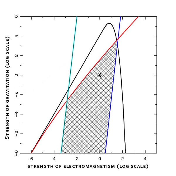
On closer examination, though, stars are remarkably robust. The strength of the electric force could vary by a factor of nearly 100 in either direction before stellar operations would be compromised. The force of gravity would have to be 100,000 times stronger. Going in the other direction, gravity could be a billion times weaker and still allow for working stars. The allowed strengths for the gravitational and electromagnetic forces depend on the nuclear reaction rate, which in turn depends on the strengths of the nuclear forces. If the reaction rate were faster, stars could function over an even wider range of strengths for gravitation and electromagnetism. Slower nuclear reactions would narrow the range.

In addition to these minimal operational requirements, stars must meet a number of other constraints that further restrict the allowed strength of the forces. They must be hot. The surface temperature of a star must be high enough to drive the chemical reactions necessary for life. In our universe, there are ample regions around most stars where planets are warm enough, about 300 kelvins, to support biology. In universes where the electromagnetic force is stronger, stars are cooler, making them less hospitable.

ADVERTISEMENT

Nautilus Members enjoy an ad-free experience. Log in or Join now .

Stars must also have long lives. The evolution of complex life forms takes place over enormous spans of time. Since life is driven by a complex ensemble of chemical reactions, the basic clock for biological evolution is set by the time scales of atoms. In other universes, these atomic clocks will tick at different rates, depending on the strength of electromagnetism, and this variation must be taken into account. When the force is weaker, stars burn their nuclear fuel faster, and their lifetimes decrease.

Finally, stars must be able to form in the first place. In order for galaxies and, later, stars to condense out of primordial gas, the gas must be able to lose energy and cool down. The cooling rate depends (yet again) on the strength of electromagnetism. If this force is too weak, gas cannot cool down fast enough and would remain diffuse instead of condensing into galaxies. Stars must also be smaller than their host galaxies—otherwise star formation would be problematic. These effects put another lower limit on the strength of electromagnetism.

Putting it all together, the strengths of the fundamental forces can vary by several orders of magnitude and still allow planets and stars to satisfy all the constraints (as illustrated in the figure below). The forces are not nearly as finely tuned as many scientists think.

Asecond example of possible fine-tuning arises in the context of carbon production. After moderately large stars have fused the hydrogen in their central cores into helium, helium itself becomes the fuel. Through a complicated set of reactions, helium is burned into carbon and oxygen. Because of their important role in nuclear physics, helium nuclei are given a special name: alpha particles. The most common nuclei are composed of one, three, four, and five alpha particles. The nucleus with two alpha particles, beryllium-8, is conspicuously absent, and for a good reason: It is unstable in our universe.

ADVERTISEMENT

Nautilus Members enjoy an ad-free experience. Log in or Join now .

The instability of beryllium creates a serious bottleneck for the creation of carbon. As stars fuse helium nuclei together to become beryllium, the beryllium nuclei almost immediately decay back into their constituent parts. At any given time, the stellar core maintains a small but transient population of beryllium. These rare beryllium nuclei can interact with helium to produce carbon. Because the process ultimately involves three helium nuclei, it is called the triple-alpha reaction. But the reaction is too slow to produce the amount of carbon observed in our universe.

To resolve this discrepancy, physicist Fred Hoyle predicted in 1953 that the carbon nucleus has to have a resonant state at a specific energy, as if it were a little bell that rang with a certain tone. Because of this resonance, the reaction rates for carbon production are much larger than they would be otherwise—large enough to explain the abundance of carbon found in our universe. The resonance was later measured in the laboratory at the predicted energy level.

The worry is that, in other universes, with alternate strengths of the forces, the energy of this resonance could be different, and stars would not produce enough carbon. Carbon production is compromised if the energy level is changed by more than about 4 percent. This issue is sometimes called the triple-alpha fine-tuning problem.

Fortunately, this problem has a simple solution. What nuclear physics takes away, it also gives. Suppose nuclear physics did change by enough to neutralize the carbon resonance. Among the possible changes of this magnitude, about half would have the side effect of making beryllium stable, so the loss of the resonance would become irrelevant. In such alternate universes, carbon would be produced in the more logical manner of adding together alpha particles one at a time. Helium could fuse into beryllium, which could then react with additional alpha particles to make carbon. There is no fine-tuning problem after all.

ADVERTISEMENT

Nautilus Members enjoy an ad-free experience. Log in or Join now .

Athird instance of potential fine-tuning concerns the simplest nuclei composed of two particles: deuterium nuclei, which contain one proton and one neutron; diprotons, consisting of two protons; and dineutrons, consisting of two neutrons. In our universe, only deuterium is stable. The production of helium takes place by first combining two protons into deuterium.

If the strong nuclear force had been even stronger, diprotons could have been stable. In this case, stars could have generated energy through the simplest and fastest of nuclear reactions, where protons combine to become diprotons and eventually other helium isotopes. It is sometimes claimed that stars would then burn through their nuclear fuel at catastrophic rates, resulting in lifetimes that are too short to support biospheres. Conversely, if the strong force had been weaker, then deuterium would be unstable, and the usual stepping stone on the pathway to heavy elements would not be available. Many scientists have speculated that the absence of stable deuterium would lead to a universe with no heavy elements at all and that such a universe would be devoid of complexity and life.

ADVERTISEMENT

Nautilus Members enjoy an ad-free experience. Log in or Join now .

As it turns out, stars are remarkably stable entities. Their structure adjusts automatically to burn nuclear fuel at exactly the right rate required to support themselves against the crush of their own gravity. If the nuclear reaction rates are higher, stars will burn their nuclear fuel at a lower central temperature, but otherwise they will not be so different. In fact, our universe has an example of this type of behavior. Deuterium nuclei can combine with protons to form helium nuclei through the action of the strong force. The cross section for this reaction, which quantifies the probability of its occurrence, is quadrillions of times larger than for ordinary hydrogen fusion. Nonetheless, stars in our universe burn their deuterium in a relatively uneventful manner. The stellar core has an operating temperature of 1 million kelvins, compared to the 15 million kelvins required to burn hydrogen under ordinary conditions. These deuterium-burning stars have cooler centers and are somewhat larger than the sun, but are otherwise unremarkable.

Similarly, if the strong nuclear force were lower, stars could continue to operate in the absence of stable deuterium. A number of different processes provide paths by which stars can generate energy and synthesize heavy elements. During the first part of their lives, stars slowly contract, their central cores grow hotter and denser, and they glow with the power output of the sun. Stars in our universe eventually become hot and dense enough to ignite nuclear fusion, but in alternative universes they could continue this contraction phase and generate power by losing gravitational potential energy. The longest-lived stars could shine with a power output roughly comparable to the sun for up to 1 billion years, perhaps long enough for biological evolution to take place.

For sufficiently massive stars, the contraction would accelerate and become a catastrophic collapse. These stellar bodies would basically go supernova. Their central temperatures and densities would increase to such large values that nuclear reactions would ignite. Many types of nuclear reactions would take place in the death throes of these stars. This process of explosive nucleosynthesis could supply the universe with heavy nuclei, in spite of the lack of deuterium.

Once such a universe produces trace amounts of heavy elements, later generations of stars have yet another option for nuclear burning. This process, called the carbon-nitrogen-oxygen cycle, does not require deuterium as an intermediate state. Instead, carbon acts as a catalyst to instigate the production of helium. This cycle operates in the interior of the sun and provides a small fraction of its total power. In the absence of stable deuterium, the carbon-nitrogen-oxygen cycle would dominate the energy generation. And this does not exhaust the options for nuclear power generation. Stars could also produce helium through a triple-nucleon process that is roughly analogous to the triple-alpha process for carbon production. Stars thus have many channels for providing both energy and complex nuclei in alternate universes.

ADVERTISEMENT

Nautilus Members enjoy an ad-free experience. Log in or Join now .

Afourth example of fine-tuning concerns the formation of galaxies and other large-scale structures. They were seeded by small density fluctuations produced in the earliest moments of cosmic time. After the universe had cooled down enough, these fluctuations started to grow stronger under the force of gravity, and denser regions eventually become galaxies and galaxy clusters. The fluctuations started with a small amplitude, denoted Q, equal to 0.00001. The primeval universe was thus incredibly smooth: The density, temperature, and pressure of the densest regions and of the most rarefied regions were the same to within a few parts per 100,000. The value of Q represents another possible instance of fine-tuning in the universe.

If Q had been lower, it would have taken longer for fluctuations to grow strong enough to become cosmic structures, and galaxies would have had lower densities. If the density of a galaxy is too low, the gas in the galaxy is unable to cool. It might not ever condense into galactic disks or coalesce into stars. Low-density galaxies are not viable habitats for life. Worse, a long enough delay might have prevented galaxies from forming at all. Beginning about 4 billion years ago, the expansion of the universe began to accelerate and pull matter apart faster than it could agglomerate—a change of pace that is usually attributed to a mysterious dark energy. If Q had been too small, it could have taken so long for galaxies to collapse that the acceleration would have started before structure formation was complete, and further growth would have been suppressed. The universe could have ended up devoid of complexity, and lifeless. In order to avoid this fate, the value of Q cannot be smaller by more than a factor of 10.

What if Q had been larger? Galaxies would have formed earlier and ended up denser. That, too, would have posed a danger for the prospects of habitability. Stars would have been much closer to one another and interacted more often. In so doing, they could have stripped planets out of their orbits and sent them hurtling into deep space. Furthermore, because stars would be closer together, the night sky would be brighter—perhaps as bright as day. If the stellar background were too dense, the combined starlight could boil the oceans of any otherwise suitable planets.

Galactic What-IfA galaxy that formed in a hypothetical universe with large initial density fluctuations might be even more hospitable than our Milky Way. The central region is too bright and hot for life, and planetary orbits are unstable. But the outer region is similar to the solar neighborhood. In between, the background starlight from the galaxy is comparable in brightness to the sunlight received by Earth, so all planets, no matter their orbits, are potentially habitable.Fred C. Adams

ADVERTISEMENT

Nautilus Members enjoy an ad-free experience. Log in or Join now .

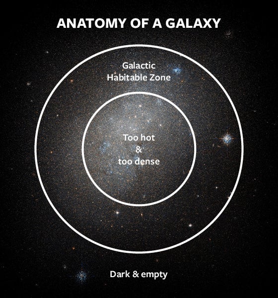
In this case, the fine-tuning argument is not very constraining. The central regions of galaxies could indeed produce such intense background radiation that all planets would be rendered uninhabitable. But the outskirts of galaxies would always have a low enough density for habitable planets to survive. An appreciable fraction of galactic real estate remains viable even when Q is thousands of times larger than in our universe. In some cases, a galaxy might be even more hospitable. Throughout much of the galaxy, the night sky could have the same brightness as the sunshine we see during the day on Earth. Planets would receive their life-giving energy from the entire ensemble of background stars rather than from just their own sun. They could reside in almost any orbit. In an alternate universe with larger density fluctuations than our own, even Pluto would get as much daylight as Miami. As a result, a moderately dense galaxy could have more habitable planets than the Milky Way.

In short, the parameters of our universe could have varied by large factors and still allowed for working stars and potentially habitable planets. The force of gravity could have been 1,000 times stronger or 1 billion times weaker, and stars would still function as long-lived nuclear burning engines. The electromagnetic force could have been stronger or weaker by factors of 100. Nuclear reaction rates could have varied over many orders of magnitude. Alternative stellar physics could have produced the heavy elements that make up the basic raw material for planets and people. Clearly, the parameters that determine stellar structure and evolution are not overly fine-tuned.

Given that our universe does not seem to be particularly fine-tuned, can we still say that our universe is the best one for life to develop? Our current understanding suggests that the answer is no. One can readily envision a universe that is friendlier to life and perhaps more logical. A universe with stronger initial density fluctuations would make denser galaxies, which could support more habitable planets than our own. A universe with stable beryllium would have straightforward channels available for carbon production and would not need the complication of the triple-alpha process. Although these issues are still being explored, we can already say that universes have many pathways for the development of complexity and biology, and some could be even more favorable for life than our own. In light of these generalizations, astrophysicists need to reexamine the possible implications of the multiverse, including the degree of fine-tuning in our universe.

ADVERTISEMENT

Nautilus Members enjoy an ad-free experience. Log in or Join now .

• Fred Adams

  Posted on January 6, 2017

  Fred Adams is a physics professor at the University of Michigan in Ann Arbor. He is the recipient of the Helen B. Warner Prize from the American Astronomical Society, the National Science Foundation Young Investigator Award, and numerous teaching awards from the University of Michigan. He is co-author of The Five Ages of the Universe: Inside the Physics of Eternity and of Origins of Existence: How Life Emerged in the Universe.

• Jackie Ferrentino

  Posted on January 6, 2017

  Jackie Ferrentino

O ajuste não tão fino do universo

Há mais de uma maneira de construir um universo adequado à vida.

• Por Fred Adams e Jackie Ferrentino
 
• 6 de janeiro de 2017
 
• Ilustrações de Jackie Ferrentino

• Compartilhar

Recupere a sensação de volta às aulas com 25% de desconto nas assinaturas da Nautilus.

O arquivo completo do Nautilus • eBooks e edições especiais • Leitura sem anúncios

Assine com 25% de desconto

Explorar

BAntes de haver vida, é preciso haver estrutura. Nosso universo sintetizou núcleos atômicos no início de sua história. Esses núcleos capturaram elétrons para formar átomos. Esses átomos se aglomeraram em galáxias, estrelas e planetas. Finalmente, os seres vivos tinham um lugar para chamar de lar. Consideramos natural que as leis da física permitam a formação de tais estruturas, mas isso não precisava ter sido o caso.

Membros do Nautilus aproveitam uma experiência sem anúncios. Entre ou cadastre-se agora .

Nas últimas décadas, muitos cientistas têm argumentado que, se as leis da física fossem, mesmo que ligeiramente, diferentes, o cosmos seria desprovido de estruturas complexas. Paralelamente, cosmólogos perceberam que o nosso universo pode ser apenas um componente do multiverso, uma vasta coleção de universos que compõe uma região muito maior do espaço-tempo. A existência de outros universos fornece uma explicação convincente para o aparente ajuste fino das leis da física. Essas leis variam de universo para universo, e vivemos em um universo que permite observadores porque não poderíamos viver em nenhum outro lugar.

Os astrofísicos têm discutido tanto o ajuste fino que muitas pessoas tomam como certo que nosso universo é preternaturalmente adequado para estruturas complexas. Até mesmo os céticos do multiverso aceitam o ajuste fino; eles simplesmente acham que deve haver alguma outra explicação. Mas, na verdade, o ajuste fino nunca foi rigorosamente demonstrado. Não sabemos realmente quais leis da física são necessárias para o desenvolvimento de estruturas astrofísicas, que por sua vez são necessárias para o desenvolvimento da vida. Trabalhos recentes sobre evolução estelar, astrofísica nuclear e formação de estruturas sugerem que o caso do ajuste fino é menos convincente do que se pensava anteriormente. Uma ampla variedade de universos possíveis poderia suportar vida. Nosso universo não é tão especial quanto parece.

TO primeiro tipo de ajuste fino envolve a intensidade das forças fundamentais da natureza em estrelas em atividade. Se a força eletromagnética fosse muito forte, a repulsão elétrica dos prótons interromperia a fusão nuclear nos núcleos estelares e as estrelas deixariam de brilhar. Se o eletromagnetismo fosse muito fraco, as reações nucleares ficariam fora de controle e as estrelas explodiriam em explosões espetaculares. Se a gravidade fosse muito forte, as estrelas ou colapsariam em buracos negros ou nunca entrariam em ignição.

ANÚNCIO

Membros do Nautilus aproveitam uma experiência sem anúncios. Entre ou cadastre-se agora .

Definindo os Parâmetros: O universo teria sido habitável mesmo se as forças do eletromagnetismo e da gravidade tivessem sido mais fortes ou mais fracas. A área hachurada mostra a faixa de valores consistentes com a vida. O asterisco mostra os valores reais em nosso universo; os eixos são escalados para esses valores. As restrições são que as estrelas devem ser capazes de sofrer fusão nuclear (abaixo da curva preta), viver o suficiente para que a vida complexa evolua (abaixo da curva vermelha), ser quentes o suficiente para suportar biosferas (à esquerda da curva azul) e não crescer mais do que suas galáxias hospedeiras (à direita da curva ciano). Fred C. Adams

Em um exame mais detalhado, porém, as estrelas são notavelmente robustas. A intensidade da força elétrica poderia variar por um fator de quase 100 em qualquer direção antes que as operações estelares fossem comprometidas. A força da gravidade teria que ser 100.000 vezes mais forte. Indo na outra direção, a gravidade poderia ser um bilhão de vezes mais fraca e ainda permitir estrelas funcionais. As intensidades permitidas para as forças gravitacional e eletromagnética dependem da taxa de reação nuclear, que por sua vez depende da intensidade das forças nucleares. Se a taxa de reação fosse mais rápida, as estrelas poderiam funcionar em uma faixa ainda maior de intensidades para gravitação e eletromagnetismo. Reações nucleares mais lentas estreitariam a faixa.

Além desses requisitos operacionais mínimos, as estrelas devem atender a uma série de outras restrições que restringem ainda mais a intensidade permitida das forças. Elas devem ser quentes. A temperatura da superfície de uma estrela deve ser alta o suficiente para conduzir as reações químicas necessárias à vida. Em nosso universo, existem amplas regiões ao redor da maioria das estrelas onde os planetas são quentes o suficiente, cerca de 300 kelvins, para sustentar a biologia. Em universos onde a força eletromagnética é mais forte, as estrelas são mais frias, o que as torna menos hospitaleiras.

ANÚNCIO

Membros do Nautilus aproveitam uma experiência sem anúncios. Entre ou cadastre-se agora .

As estrelas também devem ter vidas longas. A evolução de formas de vida complexas ocorre ao longo de enormes períodos de tempo. Como a vida é impulsionada por um conjunto complexo de reações químicas, o relógio básico para a evolução biológica é definido pelas escalas de tempo dos átomos. Em outros universos, esses relógios atômicos funcionarão em velocidades diferentes, dependendo da intensidade do eletromagnetismo, e essa variação deve ser levada em consideração. Quando a intensidade é mais fraca, as estrelas queimam seu combustível nuclear mais rapidamente e seu tempo de vida diminui.

Por fim, as estrelas devem ser capazes de se formar. Para que galáxias e, posteriormente, estrelas se condensem a partir do gás primordial, o gás deve ser capaz de perder energia e resfriar. A taxa de resfriamento depende (mais uma vez) da intensidade do eletromagnetismo. Se essa intensidade for muito fraca, o gás não consegue resfriar rápido o suficiente e permaneceria difuso em vez de se condensar em galáxias. As estrelas também devem ser menores do que suas galáxias hospedeiras — caso contrário, a formação estelar seria problemática. Esses efeitos impõem outro limite inferior à intensidade do eletromagnetismo.

Somando tudo isso, as intensidades das forças fundamentais podem variar em várias ordens de magnitude e ainda assim permitir que planetas e estrelas satisfaçam todas as restrições (como ilustrado na figura abaixo). As forças não são tão finamente ajustadas quanto muitos cientistas pensam.

UMO segundo exemplo de possível ajuste fino surge no contexto da produção de carbono. Após estrelas moderadamente grandes fundirem o hidrogênio em seus núcleos centrais em hélio, o próprio hélio se torna o combustível. Por meio de um complexo conjunto de reações, o hélio é queimado em carbono e oxigênio. Devido ao seu importante papel na física nuclear, os núcleos de hélio recebem um nome especial: partículas alfa. Os núcleos mais comuns são compostos por uma, três, quatro e cinco partículas alfa. O núcleo com duas partículas alfa, berílio-8, está notavelmente ausente, e por um bom motivo: ele é instável em nosso universo.

ANÚNCIO

Membros do Nautilus aproveitam uma experiência sem anúncios. Entre ou cadastre-se agora .

A instabilidade do berílio cria um sério gargalo para a criação de carbono. À medida que as estrelas fundem núcleos de hélio para formar berílio, os núcleos de berílio decaem quase imediatamente de volta às suas partes constituintes. A qualquer momento, o núcleo estelar mantém uma população pequena, porém transitória, de berílio. Esses raros núcleos de berílio podem interagir com o hélio para produzir carbono. Como o processo envolve, em última análise, três núcleos de hélio, é chamado de reação triplo-alfa. Mas a reação é lenta demais para produzir a quantidade de carbono observada em nosso universo.

Para resolver essa discrepância, o físico Fred Hoyle previu em 1953 que o núcleo de carbono precisa ter um estado ressonante em uma energia específica, como se fosse um pequeno sino que tocasse com um determinado tom. Devido a essa ressonância, as taxas de reação para a produção de carbono são muito maiores do que seriam de outra forma — grandes o suficiente para explicar a abundância de carbono encontrada em nosso universo. A ressonância foi posteriormente medida em laboratório no nível de energia previsto.

A preocupação é que, em outros universos, com intensidades alternadas das forças, a energia dessa ressonância poderia ser diferente, e as estrelas não produziriam carbono suficiente. A produção de carbono fica comprometida se o nível de energia for alterado em mais de 4%. Esse problema às vezes é chamado de problema do ajuste fino do triplo-alfa.

Felizmente, esse problema tem uma solução simples. O que a física nuclear tira, ela também dá. Suponha que a física nuclear mudasse o suficiente para neutralizar a ressonância do carbono. Entre as possíveis mudanças dessa magnitude, cerca de metade teria o efeito colateral de tornar o berílio estável, de modo que a perda da ressonância se tornaria irrelevante. Em tais universos alternativos, o carbono seria produzido da maneira mais lógica de adicionar partículas alfa, uma de cada vez. O hélio poderia se fundir em berílio, que poderia então reagir com partículas alfa adicionais para formar carbono. Afinal, não há problema de ajuste fino.

ANÚNCIO

Membros do Nautilus aproveitam uma experiência sem anúncios. Entre ou cadastre-se agora .

UMO terceiro exemplo de ajuste fino potencial diz respeito aos núcleos mais simples, compostos por duas partículas: núcleos de deutério, que contêm um próton e um nêutron; diprótons, compostos por dois prótons; e dineutrons, compostos por dois nêutrons. Em nosso universo, apenas o deutério é estável. A produção de hélio ocorre pela combinação inicial de dois prótons em deutério.

Se a força nuclear forte tivesse sido ainda mais forte, os diprótons poderiam ter sido estáveis. Nesse caso, as estrelas poderiam ter gerado energia por meio das reações nucleares mais simples e rápidas, nas quais os prótons se combinam para se tornarem diprótons e, eventualmente, outros isótopos de hélio. Às vezes, afirma-se que as estrelas queimariam seu combustível nuclear a taxas catastróficas, resultando em tempos de vida muito curtos para sustentar biosferas. Por outro lado, se a força forte tivesse sido mais fraca, o deutério seria instável e o trampolim usual no caminho para os elementos pesados não estaria disponível. Muitos cientistas especularam que a ausência de deutério estável levaria a um universo sem elementos pesados e que tal universo seria desprovido de complexidade e vida.

ANÚNCIO

Membros do Nautilus aproveitam uma experiência sem anúncios. Entre ou cadastre-se agora .

Acontece que as estrelas são entidades notavelmente estáveis. Sua estrutura se ajusta automaticamente para queimar combustível nuclear exatamente na taxa correta necessária para se sustentarem contra o impacto de sua própria gravidade. Se as taxas de reação nuclear forem maiores, as estrelas queimarão seu combustível nuclear a uma temperatura central mais baixa, mas, fora isso, não serão tão diferentes. De fato, nosso universo tem um exemplo desse tipo de comportamento. Núcleos de deutério podem se combinar com prótons para formar núcleos de hélio por meio da ação da força forte. A seção transversal dessa reação, que quantifica a probabilidade de sua ocorrência, é quatrilhões de vezes maior do que a da fusão de hidrogênio comum. No entanto, as estrelas em nosso universo queimam seu deutério de maneira relativamente tranquila. O núcleo estelar tem uma temperatura operacional de 1 milhão de kelvins, em comparação com os 15 milhões de kelvins necessários para queimar hidrogênio em condições normais. Essas estrelas que queimam deutério têm centros mais frios e são um pouco maiores que o Sol, mas, de resto, não apresentam características notáveis.

Da mesma forma, se a força nuclear forte fosse menor, as estrelas poderiam continuar a operar na ausência de deutério estável. Vários processos diferentes fornecem caminhos pelos quais as estrelas podem gerar energia e sintetizar elementos pesados. Durante a primeira parte de suas vidas, as estrelas se contraem lentamente, seus núcleos centrais ficam mais quentes e densos, e elas brilham com a potência do Sol. Estrelas em nosso universo eventualmente se tornam quentes e densas o suficiente para iniciar a fusão nuclear, mas em universos alternativos elas poderiam continuar essa fase de contração e gerar energia perdendo energia potencial gravitacional. As estrelas de vida mais longa poderiam brilhar com uma potência aproximadamente comparável à do Sol por até 1 bilhão de anos, talvez tempo suficiente para que a evolução biológica ocorra.

Para estrelas suficientemente massivas, a contração se aceleraria e se tornaria um colapso catastrófico. Esses corpos estelares basicamente se tornariam supernovas. Suas temperaturas e densidades centrais aumentariam a valores tão altos que reações nucleares se inflamariam. Muitos tipos de reações nucleares ocorreriam na agonia dessas estrelas. Esse processo de nucleossíntese explosiva poderia suprir o universo com núcleos pesados, apesar da falta de deutério.

Uma vez que tal universo produz quantidades vestigiais de elementos pesados, gerações posteriores de estrelas têm ainda outra opção para a queima nuclear. Este processo, chamado de ciclo carbono-nitrogênio-oxigênio, não requer deutério como um estado intermediário. Em vez disso, o carbono atua como um catalisador para instigar a produção de hélio. Este ciclo opera no interior do Sol e fornece uma pequena fração de sua energia total. Na ausência de deutério estável, o ciclo carbono-nitrogênio-oxigênio dominaria a geração de energia. E isso não esgota as opções para geração de energia nuclear. As estrelas também poderiam produzir hélio através de um processo de triplo núcleon que é aproximadamente análogo ao processo triplo-alfa para produção de carbono. As estrelas, portanto, têm muitos canais para fornecer energia e núcleos complexos em universos alternativos.

ANÚNCIO

Membros do Nautilus aproveitam uma experiência sem anúncios. Entre ou cadastre-se agora .

UMO quarto exemplo de ajuste fino diz respeito à formação de galáxias e outras estruturas de grande escala. Elas foram semeadas por pequenas flutuações de densidade produzidas nos primeiros momentos do tempo cósmico. Depois que o universo esfriou o suficiente, essas flutuações começaram a ficar mais fortes sob a força da gravidade, e regiões mais densas eventualmente se tornaram galáxias e aglomerados de galáxias. As flutuações começaram com uma pequena amplitude, denotada por Q , igual a 0,00001. O universo primordial era, portanto, incrivelmente suave: a densidade, a temperatura e a pressão das regiões mais densas e das regiões mais rarefeitas eram as mesmas com uma precisão de algumas partes por 100.000. O valor de Q representa outra possível instância de ajuste fino no universo.

Se Q tivesse sido menor, levaria mais tempo para que as flutuações se tornassem fortes o suficiente para se tornarem estruturas cósmicas, e as galáxias teriam densidades menores. Se a densidade de uma galáxia for muito baixa, o gás na galáxia não consegue resfriar. Ele pode nunca se condensar em discos galácticos ou coalescer em estrelas. Galáxias de baixa densidade não são habitats viáveis para a vida. Pior ainda, um atraso longo o suficiente poderia ter impedido a formação de galáxias. Começando há cerca de 4 bilhões de anos, a expansão do universo começou a acelerar e a separar a matéria mais rápido do que ela conseguia se aglomerar — uma mudança de ritmo que geralmente é atribuída a uma misteriosa energia escura. Se Q tivesse sido muito pequeno, poderia ter levado tanto tempo para as galáxias colapsarem que a aceleração teria começado antes que a formação da estrutura estivesse completa, e o crescimento posterior teria sido suprimido. O universo poderia ter acabado desprovido de complexidade e sem vida. Para evitar esse destino, o valor de Q não pode ser menor em mais de um fator de 10.

E se Q tivesse sido maior? As galáxias teriam se formado mais cedo e se tornado mais densas. Isso também representaria um risco para as perspectivas de habitabilidade. As estrelas estariam muito mais próximas umas das outras e interagiriam com mais frequência. Ao fazer isso, elas poderiam ter arrancado planetas de suas órbitas e lançado-os para o espaço profundo. Além disso, como as estrelas estariam mais próximas, o céu noturno seria mais brilhante — talvez tão brilhante quanto o dia. Se o fundo estelar fosse muito denso, a luz estelar combinada poderia ferver os oceanos de quaisquer planetas que, de outra forma, seriam adequados.

E se a galáxia se formasse em um universo hipotético com grandes flutuações iniciais de densidade? Uma galáxia formada em um universo hipotético com grandes flutuações iniciais de densidade poderia ser ainda mais hospitaleira do que a nossa Via Láctea. A região central é muito brilhante e quente para a vida, e as órbitas planetárias são instáveis. Mas a região externa é semelhante à vizinhança solar. No meio, a luz estelar de fundo da galáxia é comparável em brilho à luz solar recebida pela Terra, portanto, todos os planetas, independentemente de suas órbitas, são potencialmente habitáveis. Fred C. Adams

ANÚNCIO

Membros do Nautilus aproveitam uma experiência sem anúncios. Entre ou cadastre-se agora .

Neste caso, o argumento do ajuste fino não é muito restritivo. As regiões centrais das galáxias poderiam de fato produzir radiação de fundo tão intensa que todos os planetas se tornariam inabitáveis. Mas as periferias das galáxias sempre teriam uma densidade baixa o suficiente para a sobrevivência de planetas habitáveis. Uma fração apreciável do espaço galáctico permanece viável mesmo quando Q é milhares de vezes maior do que em nosso universo. Em alguns casos, uma galáxia pode ser ainda mais hospitaleira. Em grande parte da galáxia, o céu noturno poderia ter o mesmo brilho que a luz do sol que vemos durante o dia na Terra. Os planetas receberiam sua energia vital de todo o conjunto de estrelas de fundo, em vez de apenas de seu próprio sol. Eles poderiam residir em quase qualquer órbita. Em um universo alternativo com flutuações de densidade maiores que o nosso, até mesmo Plutão receberia tanta luz do dia quanto Miami. Como resultado, uma galáxia moderadamente densa poderia ter mais planetas habitáveis do que a Via Láctea.

EUEm suma, os parâmetros do nosso universo poderiam ter variado por grandes fatores e ainda permitir a existência de estrelas funcionais e planetas potencialmente habitáveis. A força da gravidade poderia ter sido 1.000 vezes mais forte ou 1 bilhão de vezes mais fraca, e as estrelas ainda funcionariam como motores nucleares de longa duração. A força eletromagnética poderia ter sido mais forte ou mais fraca por fatores de 100. As taxas de reação nuclear poderiam ter variado em muitas ordens de magnitude. A física estelar alternativa poderia ter produzido os elementos pesados que constituem a matéria-prima básica para planetas e pessoas. Claramente, os parâmetros que determinam a estrutura e a evolução estelar não são excessivamente precisos.

Dado que nosso universo não parece ser particularmente bem ajustado, ainda podemos dizer que ele é o melhor para o desenvolvimento da vida? Nossa compreensão atual sugere que a resposta é não. Podemos facilmente imaginar um universo mais favorável à vida e talvez mais lógico. Um universo com flutuações de densidade inicial mais fortes produziria galáxias mais densas, que poderiam suportar mais planetas habitáveis do que o nosso. Um universo com berílio estável teria canais diretos disponíveis para a produção de carbono e não precisaria da complicação do processo triplo-alfa. Embora essas questões ainda estejam sendo exploradas, já podemos dizer que os universos têm muitos caminhos para o desenvolvimento da complexidade e da biologia, e alguns podem ser ainda mais favoráveis à vida do que o nosso. À luz dessas generalizações, os astrofísicos precisam reexaminar as possíveis implicações do multiverso, incluindo o grau de ajuste fino em nosso universo.

ANÚNCIO

Membros do Nautilus aproveitam uma experiência sem anúncios. Entre ou cadastre-se agora .

• Fred Adams

  Publicado em6 de janeiro de 2017

  Fred Adams é professor de física na Universidade de Michigan em Ann Arbor. Recebeu o Prêmio Helen B. Warner da Sociedade Astronômica Americana, o Prêmio Jovem Pesquisador da Fundação Nacional de Ciências e diversos prêmios de ensino da Universidade de Michigan. É coautor de " As Cinco Eras do Universo: Por Dentro da Física da Eternidade" e de " Origens da Existência: Como a Vida Surgiu no Universo" .

• Jackie Ferrentino

  Publicado em6 de janeiro de 2017

  Jackie Ferrentino

•